十派的玩具箱

从分词开始，搭建起Transformer架构。

edit time: 2026-02-03 17:35:29 开始配置环境√
edit time: 2026-02-03 17:56:45 下数据集，读文档√
edit time: 2026-02-03 18:47:24 BPE先到2.4停一下
edit time: 2026-02-09 18:30:51 BPE过3/3的demo√ 没优化居然就能过
edit time: 2026-02-09 21:37:52 想把3 Transformer结构做掉
edit time: 2026-02-09 22:36:31 3.1-3.3介绍√ 后面3.4-3.6就是纯代码了，基本上是自己写一遍，再让ai写一遍，补一些细节
edit time: 2026-02-11 22:54:59 读test_model，照猫画虎Linear, Embedding, RMSNorm, SwiGLU√
edit time: 2026-02-12 23:26:05 完成整个3 Transformer结构部分√
edit time: 2026-02-13 21:36:29 完成4 Utils部分√
edit time: 2026-02-13 22:25:45 粗略地过了5 Training Loop部分，最后合在一起因为没有做tokenizer所以先搁置
edit time: 2026-03-10 09:03:18 补完训练部分√ 不管干什么，都先在PyTorch里面干一下，就知道了。

作业目录：

1. BPE tokenizer
2. Transformer LM
3. The cross-entropy loss function and the AdamW optimizer
4. The training loop (support: serilizing, loading model, optimizer state)

提到的工具：

工具	备注
cProfile	CPU性能分析工具。
torch.profiler	GPU性能分析工具。
einops	好用的重排tensor、tensor乘法、tensor聚合的可读实现库。
WanDB	日志工具，用于记录loss、acc变化，以及记录实验信息。

4 Training a Transformer LM

我们要做什么？实现一些训练Transformer必要的工具。

4.1 Cross-entropy loss

实现交叉熵损失。

4.2 The SGD Optimizer

基础的随机梯度下降优化器的原理。

4.3 AdamW

更进一步，实现AdamW优化器。

4.4 Learning rate scheduling

cosine学习率调度。

4.5 Gradient clipping

梯度裁剪，防止梯度过大。

CrossEntropyLoss

跨各个token，跨batch的平均损失。
慢慢推一下维度：
inputs: Float[Tensor, " batch_size vocab_size"]
targets: Int[Tensor, " batch_size"]
所以为了数值稳定，我们将 inputs: (batch, vocab_size) 减去它跨 vocab 维度的 max_vals: (batch, 1) ，得到 inputs_stable: (batch, vocab_size) ，
然后对 inputs_stable 执行log_sum_exp。
具体而言，先整体exp，然后在vocab_size维上做sum，最后再log。

再接下来，我们根据targets提供的标签知道了inputs中哪些是正确的，把正确的取出。

总之，其实就是算了这两部分：

$CrossEntropy(x,y)=-\log(\frac{e^{x_y}}{\sum_j e^{x_j}})=\log(\sum_j e^{x_j})-x_y$

class CrossEntropyLoss(nn.Module):
    def __init__(self):
        super().__init__()

    def forward(self, inputs, targets):
        # 1) calc log-sum-exp
        # batch "1" since 1 only automatically added in the front
        max_vals = reduce(inputs, 'batch vocab -> batch 1', reduction='max')
        inputs_stable = inputs - max_vals # (batch, vocab)
        # subtract, for numerical stability
        
        log_sum_exp = reduce(
            inputs_stable.exp(),
            'batch vocab -> batch',
            reduction='sum'
        ).log() + max_vals
        # add, for numerical stability
        
        # 2) get the predicted vals for correct labels
        # eg. targets = torch.tensor([2, 0, 3])
        # logits = torch.tensor([
        #     [0.1, 0.2, '0.3', 0.4, 0.5],
        #     ['1.0', 1.1, 1.2, 1.3, 1.4],
        #     [2.0, 2.1, 2.2, '2.3', 2.4]
        # ])
        # we take torch.tensor([0.3, 1.0, 2.3])
        target_logits = inputs.gather(
            dim=-1,
            index=targets.unsqueeze(-1)
        ).squeeze(-1)

        # 3) calc batch mean loss
        losses = log_sum_exp - target_logits
        return losses.mean()

SGD

大名鼎鼎的随机梯度下降（Stochastic Gradient Descent）。
介绍了parameter group的概念，表示模型的不同部分的参数使用不同的超参数。
用了一个简单的例子来测试超参数的影响：

from collections.abc import Callable, Iterable
from typing import Optional
import torch
import math

class SGD(torch.optim.Optimizer):
    """
    Stochastic Gradient Descent (SGD).

    eg.

    weights = torch.nn.Parameter(5 * torch.randn((10, 10)))
    opt = SGD([weights], lr=1)
    for t in range(100):
        opt.zero_grad() # Reset the gradients for all learnable parameters.
        loss = (weights**2).mean() # Compute a scalar loss value.
        print(loss.cpu().item())
        loss.backward() # Run backward pass, which computes gradients.
        opt.step() # Run optimizer step.

    Forward, compute the loss.
    Backward, compute the gradient.
    Run optimizer step, update the params.
    """

    def __init__(self, params, lr=1e-3):
        if lr < 0:
            raise ValueError(f"Invalid learning rate: {lr}")
        defaults = {"lr": lr}
        super().__init__(params, defaults)
    
    def step(self, closure: Optional[Callable] = None):
        loss = None if closure is None else closure()
        for group in self.param_groups:
            lr = group["lr"]
            for p in group["params"]:
                if p.grad is None:
                    continue

                state = self.state[p]
                t = state.get("t", 0) # iteration number we maintain
                grad = p.grad.data
                # the learning rate decays over training
                p.data -= lr / math.sqrt(t + 1) * grad
                state["t"] = t + 1

        return loss
        
weights = torch.nn.Parameter(5 * torch.randn((10, 10)))
opt = SGD([weights], lr=1)
for t in range(100):
  opt.zero_grad() # Reset the gradients for all learnable parameters.
  loss = (weights**2).mean() # Compute a scalar loss value.
  print(loss.cpu().item())
  loss.backward() # Run backward pass, which computes gradients.
  opt.step() # Run optimizer step.

结果大致如下：
可见，lr增大时，loss的值大致下降变快，直到无穷小。
但lr很大时（1e3），loss的值反倒发散到无穷大。

# lr=1
24.955036163330078 23.966821670532227 23.29372787475586 22.758888244628906 22.305986404418945 ...

# lr=1e1
20.56572723388672 13.162065505981445 9.702513694763184 7.591179847717285 6.148856163024902 ...

# lr=1e2
23.596664428710938 23.596660614013672 4.04854679107666 0.09689083695411682 1.5798126642781223e-16 ...

# lr=1e3
27.495254516601562 9925.787109375 1714339.5 190701984.0 15446859776.0

我觉得ai给了一个特别直观的解释。
想象你在一个碗状的山谷（最小值在谷底）：

• lr太小：像老太太挪步，半天走不到谷底
• lr合适：正常步伐，稳步下降
• lr偏大：大步流星，很快接近谷底
• lr过大：一步跨到对面山坡，再一步跨回来，每一步都跳到更高的地方，最终飞出碗外

AdamW

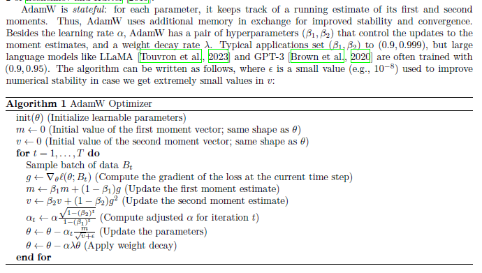
这个看起来像是在SGD的基础上加了一些数学原理的估计，使得它有很好的效果。
具体原理暂时不关心，我希望更侧重对大模型训练整体及其实现的把握。以后写到AdamW了再回过来补充原理。

class AdamW(torch.optim.Optimizer):

    def __init__(self, params, lr=1e-3, betas=(0.9, 0.999), eps=1e-8, weight_decay=0.01):
        defaults = dict(lr=lr, betas=betas, eps=eps, weight_decay=weight_decay)
        super().__init__(params, defaults)
    
    def step(self, closure=None):
        loss = None
        if closure is not None:
            loss = closure()
        
        for group in self.param_groups:
            beta1, beta2 = group['betas']
            lr = group['lr']
            eps = group['eps']
            weight_decay = group['weight_decay']
            
            for p in group['params']:
                if p.grad is None:
                    continue
                
                grad = p.grad.data
                
                # 初始化状态
                state = self.state[p]
                if len(state) == 0:
                    state['step'] = 0
                    state['m'] = torch.zeros_like(p.data)  # 一阶矩
                    state['v'] = torch.zeros_like(p.data)  # 二阶矩
                
                # 更新步数
                state['step'] += 1
                t = state['step']
                
                # 更新矩估计
                state['m'].mul_(beta1).add_(grad, alpha=1 - beta1)
                state['v'].mul_(beta2).addcmul_(grad, grad, value=1 - beta2)
                
                # 偏差修正
                bias_correction1 = 1 - beta1 ** t
                bias_correction2 = 1 - beta2 ** t
                
                # Adam更新
                denom = state['v'].sqrt().add_(eps)
                step_size = lr * (bias_correction2 ** 0.5) / bias_correction1
                p.data.addcdiv_(state['m'], denom, value=-step_size)
                
                # 权重衰减（解耦）
                if weight_decay != 0:
                    p.data.add_(p.data, alpha=-lr * weight_decay)
        
        return loss
        
        

def get_adamw_cls() -> Any:
    """
    Returns a torch.optim.Optimizer that implements AdamW.
    """
    return model.AdamW

以下是GPT对问题的回答（未检验，很可能有问题）。
之后会专门写一篇blog替换掉这里对激活值等的计算。

---

(a) AdamW 训练的内存占用分析

假设使用 float32（4字节），d_ff = 4 × d_model，batch_size = B，context_length = L。

1. 参数量与内存

组件	参数量公式	内存 (字节)
Token Embedding	V × d_model	4Vd_model
每层 Attention QKV	3 × d_model²	12d_model²
每层 Attention O	d_model²	4d_model²
每层 FFN w1/w3	2 × d_model × 4d_model = 8d_model²	32d_model²
每层 FFN w2	4d_model × d_model = 4d_model²	16d_model²
每层 RMSNorm	2 × d_model	8d_model
每层小计		12+4+32+16 = 64d_model² + 8d_model
num_layers层		N(64d_model² + 8d_model)
Final RMSNorm	d_model	4d_model
LM Head	V × d_model	4Vd_model

参数内存总量：

M_params = 8Vd_model + N(64d_model² + 8d_model) + 4d_model ≈ 8Vd_model + 64N d_model²

2. 梯度内存

梯度与参数形状相同，因此：

M_grads = M_params

3. 优化器状态内存

AdamW为每个参数存储：

• 一阶矩 m（float32）
• 二阶矩 v（float32）

因此：

M_optim = 2 × M_params

4. 激活值内存（单层）

Attention子层：

• Q/K/V投影输出：3 × B × L × d_model → 12BLd_model
• QK^T 分数矩阵：B × num_heads × L × L → 4BHL²
• Softmax输出（与分数矩阵同形状）：4BHL²
• 加权和输出：B × L × d_model → 4BLd_model
• O投影输出：B × L × d_model → 4BLd_model

FFN子层：

• w1/w3投影输出：2 × B × L × 4d_model → 32BLd_model
• SiLU输出（与w1同形状）：16BLd_model
• w2投影输出：B × L × d_model → 4BLd_model

RMSNorm（两个）：2 × B × L × d_model → 8BLd_model

单层激活值总量：

M_act_layer = (12+4+4+4+32+16+4+8)BLd_model + 8BHL²
            = 84BLd_model + 8BHL²

所有层（需要存储所有层的激活值用于反向传播）：

M_act = N × M_act_layer = 84N BLd_model + 8N BHL²

5. 输出层激活值

• Final Norm输出：B × L × d_model → 4BLd_model
• LM Head输出：B × L × V → 4BLV
• Cross-entropy中间值（log_softmax）：B × L × V → 4BLV

输出层激活值：

M_act_out = 4BLd_model + 8BLV

6. 总内存

M_total = M_params + M_grads + M_optim + M_act + M_act_out
        = M_params + M_params + 2M_params + M_act + M_act_out
        = 4M_params + M_act + M_act_out
        = 4(8Vd_model + 64N d_model²) + (84N BLd_model + 8N BHL²) + (4BLd_model + 8BLV)
        = 32Vd_model + 256N d_model² + 84N BLd_model + 8N BHL² + 4BLd_model + 8BLV

---

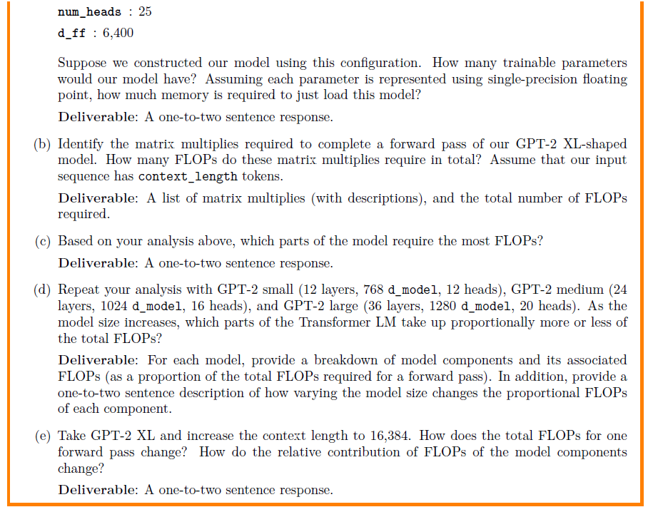
(b) GPT-2 XL 数值实例

GPT-2 XL配置：

• V = 50,257
• L = 1,024
• N = 48
• d_model = 1,600
• num_heads = 25
• H = 25
• d_ff = 6,400 = 4 × 1,600

代入公式（单位：字节）：

M_params = 8×50257×1600 + 48×64×1600²
         = 643,289,600 + 48 × 163,840,000
         = 643M + 7,864M
         = 8.507GB

M_optim = 2 × M_params = 17.014GB
M_grads = M_params = 8.507GB

M_act = 48×84×B×1024×1600 + 48×8×B×25×1024²
      = 48×84×B×1,638,400 + 48×8×B×25×1,048,576
      = 48×137,625,600×B + 48×209,715,200×B
      = 6.606B×B + 10.066B×B
      = 16.672B GB

M_act_out = 4×B×1024×1600 + 8×B×1024×50257
          = 6,553,600×B + 411,697,664×B
          = 0.0061B + 0.383B
          = 0.389B GB

总内存：

M_total = 8.507 + 17.014 + 8.507 + 16.672B + 0.389B
        = 34.028 + 17.061B GB

最大batch size（80GB内存）：

80 = 34.028 + 17.061B
17.061B = 45.972
B = 2.69 ≈ 2

答案：M_total = 34.028 + 17.061B GB，最大batch size为 2。

---

(c) AdamW 一步的FLOPs

AdamW的主要操作：

1. 更新一阶矩：m = β1·m + (1-β1)·g → 2次乘加/参数
2. 更新二阶矩：v = β2·v + (1-β2)·g² → 2次乘加 + 1次乘法/参数
3. 计算修正因子：1-β1ᵗ、1-β2ᵗ → 忽略（每步一次）
4. 参数更新：θ -= α·m/(√v+ε) → 1次除法 + 1次平方根 + 1次乘法/参数
5. 权重衰减：θ -= α·λ·θ → 1次乘加/参数

粗略估计，每个参数约 10-12 FLOPs。

总FLOPs：

F_adamw ≈ 12 × (参数量) = 12 × (8Vd_model + 64N d_model²)

对于GPT-2 XL：

参数量 ≈ 2.046B
F_adamw ≈ 12 × 2.046B = 24.55B FLOPs

---

(d) 训练时间估算

GPT-2 XL参数量 ≈ 2.046B

前向FLOPs（从之前计算）：

F_forward ≈ 4.51T FLOPs

反向FLOPs（假设是前向的2倍）：

F_backward = 2 × F_forward = 9.02T FLOPs

一步总FLOPs：

F_step = F_forward + F_backward + F_adamw
       = 4.51T + 9.02T + 0.0245T
       = 13.5545T FLOPs

A100峰值：19.5 TFLOPS
50% MFU：9.75 TFLOPS

每秒处理步数：

steps_per_sec = 9.75T / 13.5545T = 0.719 步/秒

400K步所需秒数：

seconds = 400,000 / 0.719 = 556,328 秒

转换为天：

days = 556,328 / (24×3600) = 556,328 / 86,400 ≈ 6.44 天

答案：约 6.4天

---

3 Transformer Language Model Architecture

我们要做什么？实现Transformer本身。

3.1 Transformer LM

对Transformer的整体直觉做了简介。

3.2 Output Normalization and Embedding

同上。提到相比于原论文，我们的实现修改为pre-norm。

3.3 Remark: Batching, Einsum and Efficient Computation

batch_size 和 sequence_length 通常置于开头，以便直接传播。有时需要利用 view,reshape,transpose 这些方法，但pytorch原生的写法有时不那么清晰。为了简便或者阅读友好等目的，推荐使用einops库。

3.4 Basic Building Blocks: Linear and Embedding Modules

介绍基础的Module。

3.5 Pre-Norm Transformer Block

实现pre-norm的transformer块。

3.6 The Full Transformer LM

实现整个Transformer模型，并且对它的参数、FLOPs做估算。

语言模型接收 (batch_size, sequence_length) （相当于接收一个序列），
生成对下一个token的归一化的概率分布 (batch_size, sequence_length, vocab_size) 。
训练语言模型时，优化预测得到的下一个token和实际下一个token的交叉熵损失。

连接主义！

知识：Resource accounting

这一部分本来在3 Training a Transformer LM最后，挪到了最前面方便查阅。
编写了一篇博客 怎么估算LLM的参数量和FLOPs？推一推、测一测 | 十派的玩具箱 ，详细整理了相关的内容，并且利用实际的包做了验证。

直觉：
随着模型变大，FFN和Attention占最主导（90%），其中FFN可能更多。
但是随着长上下文变长，到一定阈值后，Attention反超FFN成为绝对主导（起码超过50%）。

Linear

Linear是一个对输入向量 x 执行 y = xW^T 操作，得到输出向量 y 的层。

ps. $xW^T$ 而不是 $Wx$ 是因为尽管我们在数学上的向量往往是列向量（ $Wx$ ），但NumPy和PyTorch的内部实现通常优先使用行向量。原因很好猜到：内存的局部性。

注意首先使用 super().__init__() ，这是接下来使用 load_state_dict 手动加载权重的基础。

首先利用 torch.empty 创建 (out_features, in_features) 的 W ，然后将它用 nn.Parameter 包装，再然后使用文档Parameter Initialization部分提到的 trunc_normal_ 进行截断处理。
对于 forward 的实际实现，这里不使用einops时应该写作 x @ W^T ，因为考虑到空间局部性， x 这样的向量一般是行向量。当然，如果我们直接使用einops.einsum，就很方便了。把那些用于并行的batch之类的维度写成 ... 即可。

import torch
import torch.nn as nn
from torch.nn.init import trunc_normal_
from math import sqrt
from einops import einsum

class Linear(nn.Module):
    '''Construct a (out_features, in_features) linear layer.
    forward: y = xW^T.
    '''

    def __init__(self, in_features, out_features, device=None, dtype=None):
        super().__init__()
        self.in_features = in_features
        self.out_features = out_features
        
        std = sqrt(2.0 / (in_features + out_features))
        self.weights = trunc_normal_(
            nn.Parameter(
                torch.empty(out_features, in_features, device=device, dtype=dtype)
            ),
            mean = 0.0,
            std = std,
            a = -3.0 * std,
            b = 3.0 * std
        )

    def forward(self, x):
        if x.device != self.weights.device:
            self.weights = self.weights.to(x.device)

        # return x @ self.weights.T
        return einsum(x, self.weights, '... in_features, out_features in_features -> ... out_features')

接下来是修改adapter。
需要用到 .load_state_dict('key': weights) 来加载权重。

from cs336_basics import bpe, model

def run_linear(
    d_in: int,
    d_out: int,
    weights: Float[Tensor, " d_out d_in"],
    in_features: Float[Tensor, " ... d_in"],
) -> Float[Tensor, " ... d_out"]:
    """
    Given the weights of a Linear layer, compute the transformation of a batched input.

    Args:
        in_dim (int): The size of the input dimension
        out_dim (int): The size of the output dimension
        weights (Float[Tensor, "d_out d_in"]): The linear weights to use
        in_features (Float[Tensor, "... d_in"]): The output tensor to apply the function to

    Returns:
        Float[Tensor, "... d_out"]: The transformed output of your linear module.
    """

    linear_layer = model.Linear(d_in, d_out)
    state_dict = {'weights': weights}
    linear_layer.load_state_dict(state_dict, strict=False)
    return linear_layer(in_features)

embedding

Embedding是一个对于输入 token_id 查表，得到它的Embedding向量的层。

from cs336_basics import bpe, model

def run_linear(
    d_in: int,
    d_out: int,
    weights: Float[Tensor, " d_out d_in"],
    in_features: Float[Tensor, " ... d_in"],
) -> Float[Tensor, " ... d_out"]:
    """
    Given the weights of a Linear layer, compute the transformation of a batched input.

    Args:
        in_dim (int): The size of the input dimension
        out_dim (int): The size of the output dimension
        weights (Float[Tensor, "d_out d_in"]): The linear weights to use
        in_features (Float[Tensor, "... d_in"]): The output tensor to apply the function to

    Returns:
        Float[Tensor, "... d_out"]: The transformed output of your linear module.
    """

    linear_layer = model.Linear(d_in, d_out)
    state_dict = {'weights': weights}
    linear_layer.load_state_dict(state_dict, strict=False)
    return linear_layer(in_features)


def run_embedding(
    vocab_size: int,
    d_model: int,
    weights: Float[Tensor, " vocab_size d_model"],
    token_ids: Int[Tensor, " ..."],
) -> Float[Tensor, " ... d_model"]:
    """
    Given the weights of an Embedding layer, get the embeddings for a batch of token ids.

    Args:
        vocab_size (int): The number of embeddings in the vocabulary
        d_model (int): The size of the embedding dimension
        weights (Float[Tensor, "vocab_size d_model"]): The embedding vectors to fetch from
        token_ids (Int[Tensor, "..."]): The set of token ids to fetch from the Embedding layer

    Returns:
        Float[Tensor, "... d_model"]: Batch of embeddings returned by your Embedding layer.
    """
    embedding_layer = model.Embedding(vocab_size, d_model)
    embedding_layer.load_state_dict({'weight': weights})
    return embedding_layer(token_ids)

def run_embedding(
    vocab_size: int,
    d_model: int,
    weights: Float[Tensor, " vocab_size d_model"],
    token_ids: Int[Tensor, " ..."],
) -> Float[Tensor, " ... d_model"]:
    """
    Given the weights of an Embedding layer, get the embeddings for a batch of token ids.

    Args:
        vocab_size (int): The number of embeddings in the vocabulary
        d_model (int): The size of the embedding dimension
        weights (Float[Tensor, "vocab_size d_model"]): The embedding vectors to fetch from
        token_ids (Int[Tensor, "..."]): The set of token ids to fetch from the Embedding layer

    Returns:
        Float[Tensor, "... d_model"]: Batch of embeddings returned by your Embedding layer.
    """
    embedding_layer = model.Embedding(vocab_size, d_model)
    embedding_layer.load_state_dict({'weight': weights})
    return embedding_layer(token_ids)

RMSNorm

RMSNorm相比于普通的层归一化，少了一步减去均值的过程。
RMS(a) 即是求标准差的过程去掉了减去均值，并且再加上 1e-5 防止underflow。

有一个注意的点：在平方之前，需要upcast成float32，防止溢出。
这也启示了我们：在torch中如果有比较大的数，可能需要upcast成float32进行计算。

class RMSNorm(nn.Module):
    """RMSNorm(a_i) = a_i * g_i / RMS(a)
    RMS(a) = \sqrt(\sum_{i=1}^{d_model} a_i^2 + eps)
    g_i: (d_model) is a learnable "gain" parameter.
    eps: 1e-5. Hyperparameter.
    """

    def __init__(self, d_model, eps = 1e-5, device=None, dtype=None):
        super().__init__()
        self.weight = nn.Parameter(torch.ones(d_model, device=device, dtype=dtype))
        self.d_model = d_model
        self.eps = 1e-5

    def forward(self, x):
        # upcast input to torch.float32
        # to prevent overflow in x^2
        in_dtype = x.dtype
        x = x.to(torch.float32)
        # mean in d_model
        rms_a = torch.sqrt(x.pow(2).mean(dim=-1, keepdim=True) + self.eps)
        result = x / rms_a * self.weight
        return result.to(in_dtype)

def run_rmsnorm(
    d_model: int,
    eps: float,
    weights: Float[Tensor, " d_model"],
    in_features: Float[Tensor, " ... d_model"],
) -> Float[Tensor, " ... d_model"]:
    """Given the weights of a RMSNorm affine transform,
    return the output of running RMSNorm on the input features.

    Args:
        d_model (int): The dimensionality of the RMSNorm input.
        eps: (float): A value added to the denominator for numerical stability.
        weights (Float[Tensor, "d_model"]): RMSNorm weights.
        in_features (Float[Tensor, "... d_model"]): Input features to run RMSNorm on. Can have arbitrary leading
            dimensions.

    Returns:
        Float[Tensor,"... d_model"]: Tensor of with the same shape as `in_features` with the output of running
        RMSNorm of the `in_features`.
    """
    rmsnorm = model.RMSNorm(d_model, eps=eps)
    rmsnorm.load_state_dict({'weight': weights})
    return rmsnorm(in_features)

RoPE

RoPE 将query向量 $q=W_qx$ 利用矩阵 $R$ 进行旋转，得到了新的向量 $q'$ 。
矩阵 $R_k^i$ 是由角度 $\theta_{i,k}$ 构造得到的旋转矩阵。角度满足以下性质：

• 当dim_position $k$ 相同时，角度 $\theta_{i,k}=\frac{i}{\Theta^{(2k-2)/d}}$ 随着位置 $i$ 线性变化。这保证了无论 token_position的绝对数值大还是小，得到的注意力分数都只依赖于相对位置的差值 $i-j$ 。
• 当token_position $i$ 相同时，角度 $\theta_{i,k}=\frac{i}{\Theta^{(2k-2)/d}}$ 变化量随着 $k$ 的增加而减少，即 $k$ 比较小时，角度变化很快，频率很高； $k$ 比较大时，角度变化很慢，频率很低。
  （其中 $\Theta$ 是常数超参数， $d$ 是维度大小，即max_seq_len）

我们可以预先计算矩阵 $R_k^i$ ，在使用时再传入query向量和token_positions。

第28行的 rearrange 是这样的作用：

class RoPE(nn.Module):
    def __init__(self, theta: float, d_k: int, max_seq_len: int, device=None):
        super().__init__()
        assert d_k % 2 == 0
        self.theta = theta
        self.d_k = d_k
        self.max_seq_len = max_seq_len

        # precalc frequencies
        # freqs[k] = Θ^(-2k/d_k) for 2k = 0, 2, ..., d_k - 2
        freqs = 1.0 / (theta ** (torch.arange(0, d_k, 2, device=device).float() / d_k))
        positions = torch.arange(max_seq_len, device=device).float()

        # Cartesian product
        angles = einsum(positions, freqs, 'seq, half -> seq half')

        self.register_buffer('cos', torch.cos(angles), persistent=False)
        self.register_buffer('sin', torch.sin(angles), persistent=False)
        
    def forward(self, x, token_positions):
        orig_dtype = x.dtype
        device = x.device

        if self.cos.device != device:
            self.cos = self.cos.to(device)
            self.sin = self.sin.to(device)

        x_reshaped = rearrange(x, '... seq (half two) -> ... seq half two', two=2)

        positions = token_positions.long()
        cos = self.cos[positions]
        sin = self.sin[positions]

        x1, x2 = x_reshaped[..., 0], x_reshaped[..., 1]
        rotated_x1 = x1 * cos - x2 * sin
        rotated_x2 = x1 * sin + x2 * cos

        x_rotated = rearrange(
            [rotated_x1, rotated_x2],
            'two ... seq half -> ... seq (half two)',
            two=2
        )
        return x_rotated.to(orig_dtype)

adapter还是一个道理，而且这个都不用 load_state_dict 了。

def run_rope(
    d_k: int,
    theta: float,
    max_seq_len: int,
    in_query_or_key: Float[Tensor, " ... sequence_length d_k"],
    token_positions: Int[Tensor, " ... sequence_length"],
) -> Float[Tensor, " ... sequence_length d_k"]:
    """
    Run RoPE for a given input tensor.

    Args:
        d_k (int): Embedding dimension size for the query or key tensor.
        theta (float): RoPE parameter.
        max_seq_len (int): Maximum sequence length to pre-cache if your implementation does that.
        in_query_or_key (Float[Tensor, "... sequence_length d_k"]): Input tensor to run RoPE on.
        token_positions (Int[Tensor, "... sequence_length"]): Tensor of shape (batch_size, sequence_length) with the token positions
    Returns:
        Float[Tensor, " ... sequence_length d_k"]: Tensor with RoPEd input.
    """
    rope = model.RoPE(theta, d_k, max_seq_len)
    with torch.no_grad():
        output = rope(in_query_or_key, token_positions)
    return output

Transformer LM

DEBUG: load_state_dict

在默认实现中，顺手加了一个权重绑定：结尾 lm_head 的权重和开头 token_embedding 的权重共享，仅仅转置。
结果这一个顺手，给我带来了比较大的麻烦：
在PyTorch中，Parameter如果同名，则它们指向同一个结构。导致我在加载时，前面加载了 token_embedding 的权重，后面加载的 lm_head 的权重覆盖了它。
这一结果是，在完成了 load_state_dict 之后，逐项比较 transformer_model.named_parameters() 和 state_dict ，发现有且仅有一项 token_embedding 不一致，最大的绝对数值大约差3.1左右。

解决这一件事情之后，成功通过了这一部分的所有用例。

class TransformerBlock(nn.Module):
    def __init__(
        self,
        d_model: int,
        num_heads: int,
        d_ff: int,
        theta: float = 10000.0,
        max_seq_len: int = 2048,
        device=None,
        dtype=None
    ):
        super().__init__()
        
        self.norm1 = RMSNorm(d_model, device=device, dtype=dtype)
        self.attention = MultiHeadSelfAttention(
            d_model, num_heads, True, theta, max_seq_len, device, dtype
        )
        
        self.norm2 = RMSNorm(d_model, device=device, dtype=dtype)
        self.ffn = SwiGLU(d_model, d_ff, device=device, dtype=dtype)
    
    def forward(self, x, token_positions=None):
        x = x + self.attention(self.norm1(x), token_positions)
        x = x + self.ffn(self.norm2(x))
        return x

class TransformerLM(nn.Module):
    """
    Transformer Language Model
    """
    
    def __init__(
        self,
        vocab_size: int,
        context_length: int,
        d_model: int,
        num_heads: int,
        d_ff: int,
        num_layers: int,
        theta: float = 10000.0,
        device=None,
        dtype=None
    ):
        super().__init__()
        self.vocab_size = vocab_size
        self.context_length = context_length
        self.d_model = d_model
        self.num_layers = num_layers
        self.num_heads = num_heads
        self.d_ff = d_ff
        self.theta = theta
        
        # Token Embedding
        self.token_embedding = Embedding(
            vocab_size, 
            d_model, 
            device=device, 
            dtype=dtype
        )
        
        # Transformer Blocks - 注意变量名改为layers以匹配adapter
        self.layers = nn.ModuleList([
            TransformerBlock(
                d_model=d_model,
                num_heads=num_heads,
                d_ff=d_ff,
                theta=theta,
                max_seq_len=context_length,
                device=device,
                dtype=dtype
            )
            for _ in range(num_layers)
        ])
        
        # Final Layer Norm
        self.final_norm = RMSNorm(
            d_model, 
            device=device, 
            dtype=dtype
        )
        
        # Output Projection (权重绑定)
        self.lm_head = Linear(
            d_model, 
            vocab_size, 
            device=device, 
            dtype=dtype
        )
        
        # 罪魁祸首, 不应该用权重绑定!
        # self.lm_head.weight = self.token_embedding.weight
    
    def forward(
        self,
        token_ids: Int[Tensor, "batch seq_len"],
        token_positions: Int[Tensor, "batch seq_len"] | None = None
    ) -> Float[Tensor, "batch seq_len vocab_size"]:
        """
        前向传播
        """
        x = self.token_embedding(token_ids)  # [batch, seq_len, d_model]
        
        for layer in self.layers:
            x = layer(x, token_positions)
        
        x = self.final_norm(x)
        logits = self.lm_head(x)  # [batch, seq_len, vocab_size]
        
        return logits
        

def run_transformer_block(
    d_model: int,
    num_heads: int,
    d_ff: int,
    max_seq_len: int,
    theta: float,
    weights: dict[str, Tensor],
    in_features: Float[Tensor, " batch sequence_length d_model"],
) -> Float[Tensor, " batch sequence_length d_model"]:
    """
    Given the weights of a pre-norm Transformer block and input features,
    return the output of running the Transformer block on the input features.

    This function should use RoPE.
    Depending on your implementation, you may simply need to pass the relevant args
    to your TransformerBlock constructor, or you may need to initialize your own RoPE
    class and pass that instead.

    Args:
        d_model (int): The dimensionality of the Transformer block input.
        num_heads (int): Number of heads to use in multi-headed attention. `d_model` must be
            evenly divisible by `num_heads`.
        d_ff (int): Dimensionality of the feed-forward inner layer.
        max_seq_len (int): Maximum sequence length to pre-cache if your implementation does that.
        theta (float): RoPE parameter.
        weights (dict[str, Tensor]):
            State dict of our reference implementation.
            The keys of this dictionary are:
            - `attn.q_proj.weight`
                The query projections for all `num_heads` attention heads.
                Shape is (d_model, d_model).
                The rows are ordered by matrices of shape (num_heads, d_k),
                so `attn.q_proj.weight == torch.cat([q_heads.0.weight, ..., q_heads.N.weight], dim=0)`.
            - `attn.k_proj.weight`
                The key projections for all `num_heads` attention heads.
                Shape is (d_model, d_model).
                The rows are ordered by matrices of shape (num_heads, d_k),
                so `attn.k_proj.weight == torch.cat([k_heads.0.weight, ..., k_heads.N.weight], dim=0)`.
            - `attn.v_proj.weight`
                The value projections for all `num_heads` attention heads.
                Shape is (d_model, d_model).
                The rows are ordered by matrices of shape (num_heads, d_v),
                so `attn.v_proj.weight == torch.cat([v_heads.0.weight, ..., v_heads.N.weight], dim=0)`.
            - `attn.output_proj.weight`
                Weight of the multi-head self-attention output projection
                Shape is (d_model, d_model).
            - `ln1.weight`
                Weights of affine transform for the first RMSNorm
                applied in the transformer block.
                Shape is (d_model,).
            - `ffn.w1.weight`
                Weight of the first linear transformation in the FFN.
                Shape is (d_model, d_ff).
            - `ffn.w2.weight`
                Weight of the second linear transformation in the FFN.
                Shape is (d_ff, d_model).
            - `ffn.w3.weight`
                Weight of the third linear transformation in the FFN.
                Shape is (d_model, d_ff).
            - `ln2.weight`
                Weights of affine transform for the second RMSNorm
                applied in the transformer block.
                Shape is (d_model,).
        in_features (Float[Tensor, "batch sequence_length d_model"]):
            Tensor to run your implementation on.

    Returns:
        Float[Tensor, "batch sequence_length d_model"] Tensor with the output of
        running the Transformer block on the input features while using RoPE.
    """

    block = model.TransformerBlock(
        d_model=d_model,
        num_heads=num_heads,
        d_ff=d_ff,
        theta=theta,
        max_seq_len=max_seq_len
    )
    
    state_dict = {
        'norm1.weight': weights['ln1.weight'],
        'norm2.weight': weights['ln2.weight'],
        'attention.W_q.weight': weights['attn.q_proj.weight'],
        'attention.W_k.weight': weights['attn.k_proj.weight'],
        'attention.W_v.weight': weights['attn.v_proj.weight'],
        'attention.W_o.weight': weights['attn.output_proj.weight'],
        'ffn.w1.weight': weights['ffn.w1.weight'],
        'ffn.w2.weight': weights['ffn.w2.weight'],
        'ffn.w3.weight': weights['ffn.w3.weight'],
    }
    
    block.load_state_dict(state_dict)
    
    batch_size, seq_len = in_features.shape[0], in_features.shape[1]
    token_positions = torch.arange(seq_len, device=in_features.device)
    token_positions = token_positions.unsqueeze(0).expand(batch_size, -1)
    
    with torch.no_grad():
        output = block(in_features, token_positions)
    
    return output


def debug_transformer_weights(model, ref_weights, num_layers):
    """
    独立调试函数：对比TransformerLM模型权重与参考权重
    
    Args:
        model: 你的TransformerLM模型实例
        ref_weights: 测试传进来的weights字典
        num_layers: 层数
    """
    print("\n" + "=" * 80)
    print("🔍 TRANSFORMER LM 权重调试")
    print("=" * 80)
    
    total_mismatches = 0
    
    # 1. Token Embedding
    print("\n【1. Token Embedding】")
    print("-" * 50)
    model_w = model.token_embedding.weight
    ref_w = ref_weights['token_embeddings.weight']
    print(f"  模型: shape {tuple(model_w.shape)}")
    print(f"  参考: shape {tuple(ref_w.shape)}")
    if model_w.shape == ref_w.shape:
        diff = (model_w - ref_w).abs().max().item()
        print(f"  ✅ 形状匹配 | 最大差异: {diff:.6f}")
        if diff < 1e-5:
            print(f"  ✅ 数值一致")
        else:
            print(f"  ⚠️ 数值差异较大")
            total_mismatches += 1
    else:
        print(f"  ❌ 形状不匹配！")
        total_mismatches += 1
    
    # 2. 遍历每一层
    for layer_idx in range(num_layers):
        print(f"\n{'='*60}")
        print(f"【2.{layer_idx} Layer {layer_idx}】")
        print(f"{'='*60}")
        
        layer = model.layers[layer_idx]
        prefix = f'layers.{layer_idx}'
        
        # ----- Attention 权重 -----
        print("\n  📍 MultiHeadSelfAttention")
        
        # Q
        model_q = layer.attention.W_q.weight
        ref_q = ref_weights[f'{prefix}.attn.q_proj.weight']
        print(f"\n    [Q]")
        print(f"      模型: {tuple(model_q.shape)}")
        print(f"      参考: {tuple(ref_q.shape)}")
        if model_q.shape == ref_q.shape:
            diff = (model_q - ref_q).abs().max().item()
            print(f"      ✅ 形状匹配 | 最大差异: {diff:.6f}")
        elif model_q.shape == ref_q.T.shape:
            diff = (model_q - ref_q.T).abs().max().item()
            print(f"      🔄 需要转置 | 转置后差异: {diff:.6f}")
            total_mismatches += 1
        else:
            print(f"      ❌ 形状不匹配 (模型{model_q.shape} vs 参考{ref_q.shape})")
            total_mismatches += 1
        
        # K
        model_k = layer.attention.W_k.weight
        ref_k = ref_weights[f'{prefix}.attn.k_proj.weight']
        print(f"\n    [K]")
        print(f"      模型: {tuple(model_k.shape)}")
        print(f"      参考: {tuple(ref_k.shape)}")
        if model_k.shape == ref_k.shape:
            diff = (model_k - ref_k).abs().max().item()
            print(f"      ✅ 形状匹配 | 最大差异: {diff:.6f}")
        elif model_k.shape == ref_k.T.shape:
            diff = (model_k - ref_k.T).abs().max().item()
            print(f"      🔄 需要转置 | 转置后差异: {diff:.6f}")
            total_mismatches += 1
        else:
            print(f"      ❌ 形状不匹配")
            total_mismatches += 1
        
        # V
        model_v = layer.attention.W_v.weight
        ref_v = ref_weights[f'{prefix}.attn.v_proj.weight']
        print(f"\n    [V]")
        print(f"      模型: {tuple(model_v.shape)}")
        print(f"      参考: {tuple(ref_v.shape)}")
        if model_v.shape == ref_v.shape:
            diff = (model_v - ref_v).abs().max().item()
            print(f"      ✅ 形状匹配 | 最大差异: {diff:.6f}")
        elif model_v.shape == ref_v.T.shape:
            diff = (model_v - ref_v.T).abs().max().item()
            print(f"      🔄 需要转置 | 转置后差异: {diff:.6f}")
            total_mismatches += 1
        else:
            print(f"      ❌ 形状不匹配")
            total_mismatches += 1
        
        # O
        model_o = layer.attention.W_o.weight
        ref_o = ref_weights[f'{prefix}.attn.output_proj.weight']
        print(f"\n    [O]")
        print(f"      模型: {tuple(model_o.shape)}")
        print(f"      参考: {tuple(ref_o.shape)}")
        if model_o.shape == ref_o.shape:
            diff = (model_o - ref_o).abs().max().item()
            print(f"      ✅ 形状匹配 | 最大差异: {diff:.6f}")
        elif model_o.shape == ref_o.T.shape:
            diff = (model_o - ref_o.T).abs().max().item()
            print(f"      🔄 需要转置 | 转置后差异: {diff:.6f}")
            total_mismatches += 1
        else:
            print(f"      ❌ 形状不匹配")
            total_mismatches += 1
        
        # ----- FFN 权重 -----
        print("\n  📍 SwiGLU")
        
        # w1
        model_w1 = layer.ffn.w1.weight
        ref_w1 = ref_weights[f'{prefix}.ffn.w1.weight']
        print(f"\n    [w1]")
        print(f"      模型: {tuple(model_w1.shape)}")
        print(f"      参考: {tuple(ref_w1.shape)}")
        if model_w1.shape == ref_w1.shape:
            diff = (model_w1 - ref_w1).abs().max().item()
            print(f"      ✅ 形状匹配 | 最大差异: {diff:.6f}")
        elif model_w1.shape == ref_w1.T.shape:
            diff = (model_w1 - ref_w1.T).abs().max().item()
            print(f"      🔄 需要转置 | 转置后差异: {diff:.6f}")
            total_mismatches += 1
        else:
            print(f"      ❌ 形状不匹配 (期望 {ref_w1.shape} 或 {ref_w1.T.shape})")
            total_mismatches += 1
        
        # w2
        model_w2 = layer.ffn.w2.weight
        ref_w2 = ref_weights[f'{prefix}.ffn.w2.weight']
        print(f"\n    [w2]")
        print(f"      模型: {tuple(model_w2.shape)}")
        print(f"      参考: {tuple(ref_w2.shape)}")
        if model_w2.shape == ref_w2.shape:
            diff = (model_w2 - ref_w2).abs().max().item()
            print(f"      ✅ 形状匹配 | 最大差异: {diff:.6f}")
        elif model_w2.shape == ref_w2.T.shape:
            diff = (model_w2 - ref_w2.T).abs().max().item()
            print(f"      🔄 需要转置 | 转置后差异: {diff:.6f}")
            total_mismatches += 1
        else:
            print(f"      ❌ 形状不匹配")
            total_mismatches += 1
        
        # w3
        model_w3 = layer.ffn.w3.weight
        ref_w3 = ref_weights[f'{prefix}.ffn.w3.weight']
        print(f"\n    [w3]")
        print(f"      模型: {tuple(model_w3.shape)}")
        print(f"      参考: {tuple(ref_w3.shape)}")
        if model_w3.shape == ref_w3.shape:
            diff = (model_w3 - ref_w3).abs().max().item()
            print(f"      ✅ 形状匹配 | 最大差异: {diff:.6f}")
        elif model_w3.shape == ref_w3.T.shape:
            diff = (model_w3 - ref_w3.T).abs().max().item()
            print(f"      🔄 需要转置 | 转置后差异: {diff:.6f}")
            total_mismatches += 1
        else:
            print(f"      ❌ 形状不匹配")
            total_mismatches += 1
        
        # ----- RMSNorm -----
        print("\n  📍 RMSNorm")
        
        # norm1
        model_norm1 = layer.norm1.weight
        ref_norm1 = ref_weights[f'{prefix}.ln1.weight']
        print(f"\n    [norm1]")
        print(f"      模型: {tuple(model_norm1.shape)}")
        print(f"      参考: {tuple(ref_norm1.shape)}")
        if model_norm1.shape == ref_norm1.shape:
            diff = (model_norm1 - ref_norm1).abs().max().item()
            print(f"      ✅ 形状匹配 | 最大差异: {diff:.6f}")
        else:
            print(f"      ❌ 形状不匹配")
            total_mismatches += 1
        
        # norm2
        model_norm2 = layer.norm2.weight
        ref_norm2 = ref_weights[f'{prefix}.ln2.weight']
        print(f"\n    [norm2]")
        print(f"      模型: {tuple(model_norm2.shape)}")
        print(f"      参考: {tuple(ref_norm2.shape)}")
        if model_norm2.shape == ref_norm2.shape:
            diff = (model_norm2 - ref_norm2).abs().max().item()
            print(f"      ✅ 形状匹配 | 最大差异: {diff:.6f}")
        else:
            print(f"      ❌ 形状不匹配")
            total_mismatches += 1
    
    # 3. Final Layer Norm
    print(f"\n{'='*60}")
    print("【3. Final Layer Norm】")
    print(f"{'='*60}")
    model_final = model.final_norm.weight
    ref_final = ref_weights['ln_final.weight']
    print(f"  模型: {tuple(model_final.shape)}")
    print(f"  参考: {tuple(ref_final.shape)}")
    if model_final.shape == ref_final.shape:
        diff = (model_final - ref_final).abs().max().item()
        print(f"  ✅ 形状匹配 | 最大差异: {diff:.6f}")
    else:
        print(f"  ❌ 形状不匹配")
        total_mismatches += 1
    
    # 4. LM Head
    print(f"\n{'='*60}")
    print("【4. LM Head】")
    print(f"{'='*60}")
    model_head = model.lm_head.weight
    ref_head = ref_weights['lm_head.weight']
    print(f"  模型: {tuple(model_head.shape)}")
    print(f"  参考: {tuple(ref_head.shape)}")
    if model_head.shape == ref_head.shape:
        diff = (model_head - ref_head).abs().max().item()
        print(f"  ✅ 形状匹配 | 最大差异: {diff:.6f}")
    elif model_head.shape == ref_head.T.shape:
        diff = (model_head - ref_head.T).abs().max().item()
        print(f"  🔄 需要转置 | 转置后差异: {diff:.6f}")
        total_mismatches += 1
    else:
        print(f"  ❌ 形状不匹配")
        total_mismatches += 1
    
    # 5. 总结
    print("\n" + "=" * 80)
    print("📊 调试总结")
    print("=" * 80)
    if total_mismatches == 0:
        print("✅ 所有权重形状匹配！")
        print("   如果输出仍然不对，检查:")
        print("   - RoPE是否生效")
        print("   - 因果掩码是否正确")
        print("   - forward是否传递了token_positions")
    else:
        print(f"❌ 发现 {total_mismatches} 处形状不匹配")
        print("   需要根据上述 🔄 标记添加 .T 转置")
    
    print("\n" + "=" * 80)

def run_transformer_lm(
    vocab_size: int,
    context_length: int,
    d_model: int,
    num_layers: int,
    num_heads: int,
    d_ff: int,
    rope_theta: float,
    weights: dict[str, Tensor],
    in_indices: Int[Tensor, " batch_size sequence_length"],
) -> Float[Tensor, " batch_size sequence_length vocab_size"]:
    """Given the weights of a Transformer language model and input indices,
    return the output of running a forward pass on the input indices.

    This function should use RoPE.

    Args:
        vocab_size (int): The number of unique items in the output vocabulary to be predicted.
        context_length (int): The maximum number of tokens to process at once.
        d_model (int): The dimensionality of the model embeddings and sublayer outputs.
        num_layers (int): The number of Transformer layers to use.
        num_heads (int): Number of heads to use in multi-headed attention. `d_model` must be
            evenly divisible by `num_heads`.
        d_ff (int): Dimensionality of the feed-forward inner layer (section 3.3).
        rope_theta (float): The RoPE $\Theta$ parameter.
        weights (dict[str, Tensor]):
            State dict of our reference implementation. {num_layers} refers to an
            integer between `0` and `num_layers - 1` (the layer index).
            The keys of this dictionary are:
            - `token_embeddings.weight`
                Token embedding matrix. Shape is (vocab_size, d_model).
            - `layers.{num_layers}.attn.q_proj.weight`
                The query projections for all `num_heads` attention heads.
                Shape is (num_heads * (d_model / num_heads), d_model).
                The rows are ordered by matrices of shape (num_heads, d_k),
                so `attn.q_proj.weight == torch.cat([q_heads.0.weight, ..., q_heads.N.weight], dim=0)`.
            - `layers.{num_layers}.attn.k_proj.weight`
                The key projections for all `num_heads` attention heads.
                Shape is (num_heads * (d_model / num_heads), d_model).
                The rows are ordered by matrices of shape (num_heads, d_k),
                so `attn.k_proj.weight == torch.cat([k_heads.0.weight, ..., k_heads.N.weight], dim=0)`.
            - `layers.{num_layers}.attn.v_proj.weight`
                The value projections for all `num_heads` attention heads.
                Shape is (num_heads * (d_model / num_heads), d_model).
                The rows are ordered by matrices of shape (num_heads, d_v),
                so `attn.v_proj.weight == torch.cat([v_heads.0.weight, ..., v_heads.N.weight], dim=0)`.
            - `layers.{num_layers}.attn.output_proj.weight`
                Weight of the multi-head self-attention output projection
                Shape is ((d_model / num_heads) * num_heads, d_model).
            - `layers.{num_layers}.ln1.weight`
                Weights of affine transform for the first RMSNorm
                applied in the transformer block.
                Shape is (d_model,).
            - `layers.{num_layers}.ffn.w1.weight`
                Weight of the first linear transformation in the FFN.
                Shape is (d_model, d_ff).
            - `layers.{num_layers}.ffn.w2.weight`
                Weight of the second linear transformation in the FFN.
                Shape is (d_ff, d_model).
            - `layers.{num_layers}.ffn.w3.weight`
                Weight of the third linear transformation in the FFN.
                Shape is (d_model, d_ff).
            - `layers.{num_layers}.ln2.weight`
                Weights of affine transform for the second RMSNorm
                applied in the transformer block.
                Shape is (d_model,).
            - `ln_final.weight`
                Weights of affine transform for RMSNorm applied to the output of the final transformer block.
                Shape is (d_model, ).
            - `lm_head.weight`
                Weights of the language model output embedding.
                Shape is (vocab_size, d_model).
        in_indices (Int[Tensor, "batch_size sequence_length"]) Tensor with input indices to run the language model on. Shape is (batch_size, sequence_length), where
            `sequence_length` is at most `context_length`.

    Returns:
        Float[Tensor, "batch_size sequence_length vocab_size"]: Tensor with the predicted unnormalized
        next-word distribution for each token.
    """
    transformer_model = model.TransformerLM(
        vocab_size=vocab_size,
        context_length=context_length,
        d_model=d_model,
        num_heads=num_heads,
        d_ff=d_ff,
        num_layers=num_layers,
        theta=rope_theta
    )
    
    state_dict = {}
    
    # Token Embedding
    state_dict['token_embedding.weight'] = weights['token_embeddings.weight']
    
    # Transformer Block
    for layer_idx in range(num_layers):
        prefix = f'layers.{layer_idx}'
        
        # attention
        state_dict[f'layers.{layer_idx}.attention.W_q.weight'] = weights[f'{prefix}.attn.q_proj.weight']
        state_dict[f'layers.{layer_idx}.attention.W_k.weight'] = weights[f'{prefix}.attn.k_proj.weight']
        state_dict[f'layers.{layer_idx}.attention.W_v.weight'] = weights[f'{prefix}.attn.v_proj.weight']
        state_dict[f'layers.{layer_idx}.attention.W_o.weight'] = weights[f'{prefix}.attn.output_proj.weight']
        
        # FFN
        w1_weight = weights[f'{prefix}.ffn.w1.weight']  # (d_ff, d_model)
        state_dict[f'layers.{layer_idx}.ffn.w1.weight'] = w1_weight  # 转置成 (d_model, d_ff)
        
        w2_weight = weights[f'{prefix}.ffn.w2.weight']  # (d_model, d_ff)
        state_dict[f'layers.{layer_idx}.ffn.w2.weight'] = w2_weight  # 转置成 (d_ff, d_model)
        
        w3_weight = weights[f'{prefix}.ffn.w3.weight']  # (d_ff, d_model)
        state_dict[f'layers.{layer_idx}.ffn.w3.weight'] = w3_weight  # 转置成 (d_model, d_ff)
        
        # RMSNorm
        state_dict[f'layers.{layer_idx}.norm1.weight'] = weights[f'{prefix}.ln1.weight']
        state_dict[f'layers.{layer_idx}.norm2.weight'] = weights[f'{prefix}.ln2.weight']
    
    state_dict['final_norm.weight'] = weights['ln_final.weight']

    lm_head_weight = weights['lm_head.weight']
    state_dict['lm_head.weight'] = lm_head_weight
    
    # 加载权重
    transformer_model.load_state_dict(state_dict, strict=False)
    # debug_transformer_weights(transformer_model, weights, num_layers) # DEBUG2
    
    # DEBUG1: 对比state_dict和named_parameters
    # for name, _ in transformer_model.named_parameters():
    #     if name in state_dict:
    #         print(f"✅ {name}")
    #     else:
    #         print(f"❌ {name} 不在state_dict中")

    # 生成位置索引
    batch_size, seq_len = in_indices.shape
    device = in_indices.device
    token_positions = torch.arange(seq_len, device=device)
    token_positions = token_positions.unsqueeze(0).expand(batch_size, -1)
    
    # 前向传播
    with torch.no_grad():
        logits = transformer_model(in_indices, token_positions)
    
    return logits

2 BPE

我们要做什么？实现基于BPE算法的分词器。

2.1 The Unicode Standard
介绍每个字符的unicode数字转换方法。在python中是 ord 和 chr 。

2.2 Unicode Encodings
介绍 .encode 和 .decode 方法，可以将字符串和unicode byte序列进行互相转换。

2.3 Subword Tokenization
介绍子词分词。

2.4 BPE Tokenizer Training
以简单的例子，介绍BPE Tokenizer的训练。（最终实现效果与 tiktoken 对齐）

2.5 Experimenting with BPE Tokenizer Training
在TinyStories数据集上进行BPE Tokenizer训练。

2.6 BPE Tokenizer: Encoding and Decoding
实现BPE Tokenizer的编码和解码。

2.7 Experiments
一些用于提升理解的问题和实验。

阅读知识部分

通过 ord 将Unicode转为int ，chr 将int转为Unicode。
可见，chr的返回值得到一个包含了相关字符的Unicode字符串。
但是，它在print中会自动进行一层解析，例如空字符0。

>>> ord('牛')
29275
>>> chr(29275)
'牛'

>>> chr(0)
'\x00'
>>> print(chr(0))

>>> "this is a test" + chr(0) + "string"
'this is a test\x00string'
>>> print("this is a test" + chr(0) + "string")
this is a teststring

不直接使用Unicode：词汇表太大，太稀疏，而且需要处理词汇表外的词。
(原始字符串) -.encode("utf-8") -> (bytes) - list() -> (list of bytes)

连着几个byte表示一个Unicode字符，那逐byte转utf-8肯定有问题了。
玩个meme

>>> decode_utf8_bytes_to_str_wrong("锟斤拷".encode("utf-8"))    
Traceback (most recent call last):
  File "<stdin>", line 1, in <module>
  File "<stdin>", line 2, in decode_utf8_bytes_to_str_wrong     
UnicodeDecodeError: 'utf-8' codec can't decode byte 0xe9 in position 0: unexpected end of data

参考 UTF-8 - Wikipedia ，每个byte的开始位是有要求的。

In UTF-8, two-byte sequences must match the pattern:

110xxxxx 10xxxxxx

所以可以构造例子 [11111111, 11111111] 不满足条件：

>>> bytes([255,255]).decode("utf-8")
Traceback (most recent call last):
  File "<stdin>", line 1, in <module>
UnicodeDecodeError: 'utf-8' codec can't decode byte 0xff in position 0: invalid start byte

（放空）
我们刚刚做的事情是把原始的字符串转化成了连续的byte：.encode("utf-8")。
现在文章的表示变得相当长，训练模型需要太多的计算。因此需要压缩。
压缩的方法是，让词汇表的数量增加（256），添加子词，实现对整个序列的压缩。构造词汇表的过程称作“训练BPE tokenizer”。

pre-tokenize：例如使用正则表达式，把空格和后面的词汇连在一起。
使用 re.finditer 。
For example, the word 'text' might be a pre-token that appears 10 times. In this case, when we count how often the characters ‘t’ and ‘e’ appear next to each other, we will see that the word ‘text’ has ‘t’ and ‘e’ adjacent and we can increment their count by 10 instead of looking through the corpus. Since we’re training a byte-level BPE model, each pre-token is represented as a sequence of UTF-8 bytes.

>>> PAT = r"""'(?:[sdmt]|ll|ve|re)| ?\p{L}+| ?\p{N}+| ?[^\s\p{L}\p{N}]+|\s+(?!\S)|\s+"""
>>> # requires `regex` package
>>> import regex as re
>>> re.findall(PAT, "some text that i'll pre-tokenize")
['some', ' text', ' that', ' i', "'ll", ' pre', '-', 'tokenize']

BPE包括三个步骤：

• Vocabulary Initialization
• Pre-tokenization
• Compute BPE merges（使用频率最高且字典序最大的）
  频率：`dict[tuple[bytes], int]

eg. pre-token的依次合并：
{low: 5, lower: 2, widest: 3, newest: 6}
{(l,o,w): 5, (l,o,w,e,r): 2, (w,i,d,e,st): 3, (n,e,w,e,st): 6}
{(l,o,w): 5, (l,o,w,e,r): 2, (w,i,d,est): 3, (n,e,w,est): 6}
Continuing this, the sequence of merges we get in the end will be ['s t', 'e st', 'o w', 'l ow', 'w est', 'n e','ne west', 'w i', 'wi d', 'wid est', 'low e', 'lowe r'] 。

此时词汇表从一开始的 [<|endoftext|>, [...256 BYTE CHARS] 变成：
[<|endoftext|>, [...256 BYTE CHARS], st, est, ow, low, west, ne]

2.4 BPE Tokenizer Training的naive实现

规划模块+逐个模块实现并检查.

对于这样一个问题，将文本文件读入、得到一个BPE tokenizer，
需要以下几部分：
(1) 读入文本，得到文本段（chunk）。
(2) GPT-2的pre-token，re.finditer ，得到一小片被pre-token过的文本。
(3) 两个数据结构：词汇表和频率表。对这样一小片文本，遍历每个字符，添加更新频率表 dict[tuple[bytes], int] 。
(4) 在频率表中取出频率最高的（通过 max ），合并 tuple[bytes] 为新的 typle[bytes] 。更新词汇表和频率表。

那么初始实现又慢又错，包括：

1. 字节级别 vs 字符串级别：你目前用字符串处理，但要求是字节级别的BPE
2. GPT-2正则表达式：需要特殊处理文本分割
3. 数据结构：vocab应该是 dict[int, bytes] 而不是 dict[int, str]
   错在没有搞懂bytes和字符的区别，慢在没有做优化（1.5s）。

首先搞懂一下字节级别BPE。动手实现和优化BPE Tokenizer的训练——第1部分：最简单实现 - 李理的博客

沉下心来，别着急，慢慢来。
仔细读test，把自己的函数行为和test搞成完全一致。

之后仔细读了一下，发现一是byte没有存对，二是split应该先按照特殊token，再使用GPT-2的分词。两个问题都解决掉就ok了。

2.7 Experiments的回答

(a) 压缩比的含义

压缩比 = 原始文本字节数 / 产生的token数量
不同tokenizer的压缩比差异：

• TinyStories tokenizer (10K vocab)：针对儿童故事训练，对简单词汇压缩比较好
• OpenWebText tokenizer (32K vocab)：更大词表，能识别更多复杂词汇和短语
  通常词表越大，压缩比越高（每个token代表更多字节），因为能匹配更长的常见词/子词单元。

(b) 用TinyStories tokenizer处理OpenWebText

会发生什么？

• 压缩比下降：很多OpenWebText中的词汇（技术术语、复杂词汇、特殊符号）在TinyStories词表中不存在，会被切成更小的子词单元
• 定性描述：文本会被"过度切分"，例如"neural network"可能变成 ["neural", "▁network"] 或者更碎，导致token序列变长
• 本质：这是领域不匹配问题——tokenizer没见过足够多的该领域词汇

下面的内容来自我实际的训练日志：

Step 1/3: train BPE tokenizer
BPE training configuration:
  input_path: data/TinyStoriesV2-GPT4-train.txt
  vocab_size: 10000
  special_tokens: ['<|endoftext|>']
  progress_every: 100
  heartbeat_seconds: 15
  vocab_out: tokenizer/tinystories_bpe_vocab.pkl
  merges_out: tokenizer/tinystories_bpe_merges.pkl
[progress] read_corpus done in 12.2s, chars=2226845268
Saved tokenizer artifacts:
  vocab_path: tokenizer/tinystories_bpe_vocab.pkl
  merges_path: tokenizer/tinystories_bpe_merges.pkl
  longest_token: b' accomplishment'
  longest_token_len: 15
  total_elapsed: 11m42.2s

估算一下，总计 2226845268 bytes ，训练BPE tokenizer总计11m42.2s， 大约就是 2226845268/702.2=3171240.76901 bytes/sec ，即大约3MB/s。
这个表现我觉得挺好了。根据 openai/tiktoken: tiktoken is a fast BPE tokeniser for use with OpenAI's models. 的说明，他们的tiktoken在同样单线程的情况下目测大约是6MB/s，在只使用了有限数量的工程优化的前提下达成这样的效果挺振奋人心的。
尽管许多工程优化的实现细节并不是完全我自己一行一行敲的 甚至low level的大部分实现几乎都不是自己一行一行敲的 ，仍然收获良多。

(c) tokenizer吞吐量估算

估算逻辑：

1. 先测量tokenizer处理一定量文本的速度（bytes/sec）
2. 用这个速率计算处理825GB所需时间
   例如：如果tokenizer速度是50 MB/sec，则825GB需要：
   825 × 1024 MB ÷ 50 MB/sec ≈ 16,896秒 ≈ 4.7小时
   实际速度取决于：

• tokenizer实现（BPE算法效率）
• 并行化程度
• 硬件（CPU/GPU）

其实这个题是要我估算，我一开始没反应过来。 感谢GPT，差点真去训了。
825GB按我的3MB/s大约就是281600s，约为78小时。 差点浪费78小时的算力。

(d) 为什么用uint16？

uint16 (无符号16位整数) 是合适选择因为：

• 取值范围够用：uint16范围 0-65535，覆盖vocab_size (10K和32K都在这个范围内)
• 存储效率高：每个token只占2字节，比int64 (8字节) 节省75%空间
• 内存友好：处理大规模数据集时，内存占用更小，加载更快
  对比：
• uint8 (0-255) 不够用（最大256 < 32K）
• uint32 浪费空间（能存40亿，但只需要3.2万）
• uint16 刚刚好

1 环境配置

Working on projects | uv

整个作业做完后感慨一下，uv真的是非常好用的工具。
我前后需要切换环境版本，uv帮我省去了相当多的环境配置的麻烦。

环境为 cs336 ，Python=3.12，在WSL中。

uv run -- flask run -p 3000
- `uv run`：uv 的命令
- `--`：分隔符，表示 "uv 的参数到此结束"
- `flask run -p 3000`：这些参数全部传递给 `flask` 命令

torch.nn — PyTorch 2.10 documentation