MiniTorch的一个实现
项目文档链接:MiniTorch
项目仓库:minitorch/minitorch: The full minitorch student suite.
我的实现:Meredith2328/minitorch: The full minitorch student suite.
(完成了Fundamentals, ML Primer, AutoDiff, Tensors, Efficiency部分,未涉及Networks部分。)
另外推荐参考这个,写得比我好得多:MiniTorch-学习全攻略.pdf
安装环境
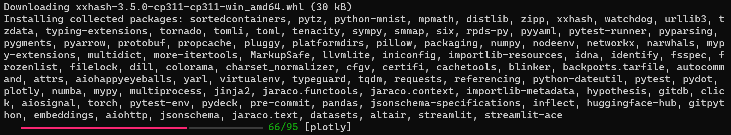
由于官方运行环境限定不够严密、部分包已发生更新,可能出现包不兼容的问题。我使用的是以下包版本。
将以下内容保存为requirements.txt并替换原始项目使用的requirements.txt和requirements.txt.extra:
backports.tarfile==1.2.0
colorama==0.4.6
datasets==2.21.0
embeddings==0.0.8
hypothesis==6.111.2
importlib-metadata==6.11.0
importlib-resources==6.4.0
jaraco.text==3.12.1
mypy==1.11.2
numba==0.60.0
plotly==5.24.0
pre-commit==3.8.0
pydot==3.0.1
pytest-env==1.1.3
pytest-runner==6.0.1
python-mnist==0.7
streamlit-ace==0.1.1
tomli==2.0.1
torch==2.4.0
numpy==1.24.0
streamlit==1.26.0
关于requirements的说明:
conda create -n myminitorch python==3.11
官方setup给的requirements有conflict,参考了pr里的requirements进行了修改
pip install -r requirements.txt
pip install -Ue .
之后发现torch版本很新、自动装的2.0的numpy不兼容,手动降级一下:
pip install numpy==1.24
以及跑Task0.5出了一些id重复的报错,判断是Streamlit版本新了一点加了检查,为了省去改代码的麻烦手动降级一下:
pip install streamlit==1.26.0

之后做到Efficiency(Task3那些)要用CUDA,我本地机CUDA==12.6,所以参考了pytorch官网的指令在环境里装gpu的pytorch:
pip3 install torch torchvision torchaudio --index-url https://download.pytorch.org/whl/cu126
Fundamentals
Fundamentals:torch的算子Operator,模块Module等。
(负责利用Python的math库,开发一些诸如sigmoid, add, mul之类的函数)
实现细节
注意true置为1.0,false置为0.0。
modern python语法:
Callable[[inputs], output]
所有输入参数传为第一个列表参数[type],输出为type,表示一个以[type]为输入参数、type为返回值的函数
def map(fn: Callable[[float], float])
-> Callable[[Iterable[float]], Iterable[float]]:
解读为:
传入一个函数参数fn,输出一个函数。
fn的性质是输入一个float,输出float。
输出函数的性质是输入一个Iterable[float]即float的列表,输出Iterable[float]。
多用assert_close而非==。
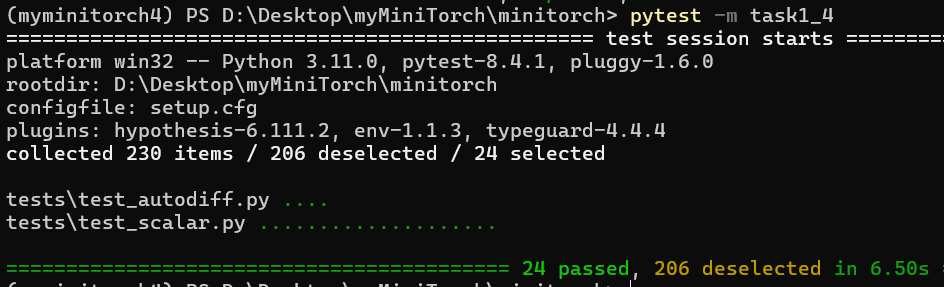
结果
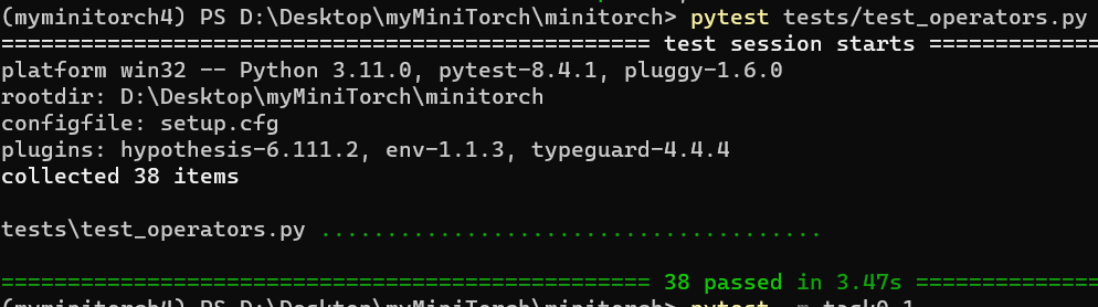
最终成功跑通:
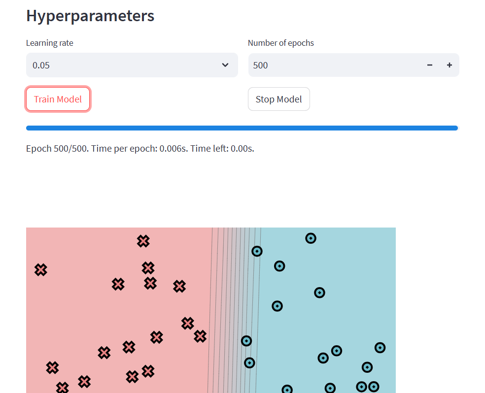
看起来streamlit是一个类似于tensorflow playground的可视化模块。
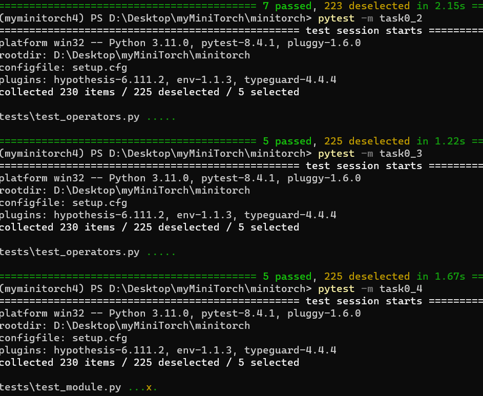
跑通task0_1到task0_4:
ps. 这里有一个实现细节:
operators.py里的函数不能相互依赖,比如sigmoid不能用同模块下的exp,但是可以用math.exp等,这是为了Efficiency一章numba能够识别相关函数。
ML Primer
ML Primer:讲了一点机器学习基础,以二分类为例,无代码作业。
文中对ReLU的理解例子十分有趣,看一看:
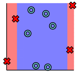
Neural networks are compound model classes that divide classification into two or more stages. Each stage uses a linear model to seperate the data. And then an activation function to reshape it.
We would like only points in the green or yellow sections to be classified as X's.
To do this, we employ an activation function that filters out only these points. This function is known as a ReLU function, which is a fancy way of saying "threshold".
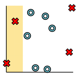
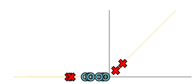
只考虑其中一个分类边界,wx+b之后进行ReLU,只保留了黄色部分的z值、而负半轴的z值置为0(ReLU正半轴,对应前述黄色部分),
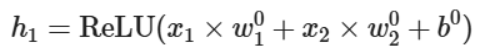
相当于对所有初始数据进行的一种变换h1得到了下述的h1值,可以把它们画到黄色轴上。

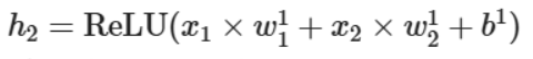
同理我们也可以对所有初始数据进行另一个变换得到h2,我们可以把它们画到上述绿色轴上。
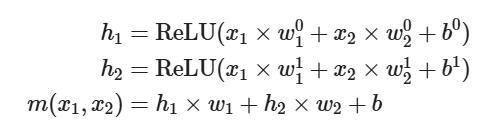
有点像是把它们降维到轴上之后就很容易划分出两个轴上的边界点,从而得到边界线,即将两个不同的变换值整合在一块的一个线性变换:

再升维回去,直接考虑整个图像的效果就得到了一个非线性的分类边界:
Mathematically we can think of the transformed data as values h1,h2 which we get from applying separators with different parameters to the original data.
The final prediction then applies a separator to h1,h2.
AutoDiff
Autodiff:标量scalar,自动求导,包括反向传播
(这时候已经能拿来跑模型训练了,但是因为没有并行所以效率很低)
AutoDiff
modern python语法:打包与解包
打包:函数内使用参数
def central_difference(f: Any, *vals: Any, arg: int = 0, epsilon: float = 1e-6) -> Any:
(这里会把中间的参数全部打包成一整个元组vals)解包:函数外传入参数
return (f(*valsAdd) - f(*valsSub)) / (2 * epsilon)
(这里需要在元组前加入解包的*符号才能传入n个参数)
注意使用中心差分,所以是 (f(x + h) - f(x - h)) / 2h 而不是我们习惯的单h求导方式
查完wiki发现这一页有写知识点hhhhhh
Scalar
Autodifferentiation works by collecting information about the computation path used within the function, and then transforming this information into a procedure for computing derivatives. Unlike the black-box method, autodifferentiation will allow us to use this information to compute each step more precisely.
需要实现跟踪计算。
所以这里的思想同样是通过每一步多记录信息、为我们整体的更优思路提供方便。
包括将数值和计算函数进行包装。
要达成的效果:
x1 = minitorch.Scalar(10)
x2 = minitorch.Scalar(30)
y = x1 + x2
y.history
ScalarHistory(last_fn=<class 'minitorch.scalar_functions.Add'>, ctx=Context(no_grad=False, saved_values=()), inputs=[Scalar(10.000000), Scalar(30.000000)])
所以这就是所谓的forward函数的作用吗。
apply除了forward中的实际操作,还记录了各种操作,便于利用。
modern python语法:类方法
在 Python 中,cls 是类方法的第一个参数,用于表示类本身。
它类似于实例方法中的 self,但 self 代表的是类的实例对象,而 cls 代表的是类对象。
- 类方法:使用 @classmethod 装饰器定义,第一个参数必须是 cls,用于访问类变量和其他类方法。
- 静态方法:使用 @staticmethod 装饰器定义,不需要 self 或 cls 参数,不能访问类变量。
class MyClass:
	class_variable = "I am a class variable"

	@staticmethod
	def static_method():
		print("I am a static method")

	@classmethod
	def class_method(cls):
		print(cls.class_variable)
之后理一下ScalarFunction的结构:
这里使用了静态类和cls上下文来组织代码。
cls是具体的类,所有类都需要在调用自身实现的forward的同时,进行统一输入类型、和创建context等操作,所以将这些统一的操作写到静态的ScalarFunction里。
这样的好处是,每个具体类都只需要关心具体的function实现,而无须考虑接口处理问题。
软件工程知识:工厂方法
定义一个工厂类(ScalarFunction),它可以根据参数的不同返回不同类的实例(apply类方法),被创建的实例通常都具有共同的父类(Scalar),这正是简单工厂模式。
(重复一遍,简单工厂模式根据不同传入参数创建不同实例。)
而将实例创建的具体逻辑不统一在工厂类、而是交予专门的工厂子类完成(如Add等),这正是更进一步的工厂方法模式。工厂类只要简单地调用工厂子类变量cls即可。
class ScalarFunction:

    @classmethod
    def _backward(cls, ctx: Context, d_out: float) -> Tuple[float, ...]:
        return wrap_tuple(cls.backward(ctx, d_out))  # type: ignore

    @classmethod
    def _forward(cls, ctx: Context, *inps: float) -> float:
	    # _forward和_backward一个解包一个装包, 规整一点, 具体逻辑留给具体类
        return cls.forward(ctx, *inps)  # type: ignore

    @classmethod
    def apply(cls, *vals: "ScalarLike") -> Scalar:
	    ...
	    # 感觉这里也可以直接调用cls.forward呢,
	    # 或许是为了代码规整,一个_forward一个_backward都写在静态类里
	    # 这样的话forward只用写具体逻辑了
        c = cls._forward(ctx, *raw_vals)
debug:
        c = cls._forward(ctx, *raw_vals)
>       assert isinstance(c, float), "Expected return type float got %s" % (type(c))
E       AssertionError: Expected return type float got <class 'int'>
E       Falsifying example: test_one_args(
E           fn=('exp', exp, exp),
E           t1=Scalar(0.000000),  # or any other generated value
E       )

minitorch\scalar_functions.py:64: AssertionError
思考:为什么c是int,为什么_forward返回了一个int。追踪!
通过给Neg加print打印类型检错,发现传入int之后加neg还是int。
在operator里加了个强制转换,解决了问题。
def forward(ctx: Context, a: float) -> float:
	# print('type of a here is ', type(a))
	# print('type of neg(a) here is ', type(operators.neg(a)))
	return operators.neg(a) # 这里需要强制加个转换, 好奇怪
type of a here is  <class 'int'>
type of neg(a) here is  <class 'int'>
def neg(x: float) -> float:
    "$f(x) = -x$"
    return -float(x)
Chain Rule
将每个函数理解成一个黑箱操作,输入了上一个黑箱的结果,函数调用层层嵌套,
每次求导就是逆黑箱的过程,输入了上一次逆黑箱的结果,求导结果依次相乘。
每次backward就是每个逆黑箱求导的具体过程,即求导并乘d_output。
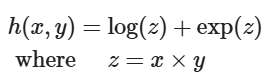
例如forward是log(a),一个输入变量a,
那么backward输出也只有结果对a求导得到的一个值再乘d_output,即d_output / a。
再例如forward是a+b,两个输入变量a和b,
那么backward输出是结果对两个变量分别求偏导得到的两个值、每个值乘d_output,即d_output和d_output。
class Log(ScalarFunction):
    "Log function $f(x) = log(x)$"

    @staticmethod
    def forward(ctx: Context, a: float) -> float:
        '''保存a, 计算log(a)并返回'''
        ctx.save_for_backward(a)
        return operators.log(a)

    @staticmethod
    def backward(ctx: Context, d_output: float) -> float:
        '''取出保存的a, 根据传回的d_output, 计算d_output/a并返回, 即d_output f\'(x)'''
        (a,) = ctx.saved_values
        return operators.log_back(a, d_output)
那么chain rule就是将层层嵌套得到的最终函数一步步逆黑箱,得到计算结果。
为了编写chain rule,我们需要每个黑箱的信息。看看history是怎么记录的。
ps. last_fn其实是当前要计算处理的function的意思,至于为什么叫last后面就知道了
    last_fn: Optional[Type[ScalarFunction]] = None
    ctx: Optional[Context] = None
    inputs: Sequence[Scalar] = ()
scalar实例是由一系列scalarFunction操作得到的。
在scalarFunction这个黑盒进行apply时将history以以下形式组织:
# Create a new variable from the result with a new history.
back = minitorch.scalar.ScalarHistory(cls, ctx, scalars)
return minitorch.scalar.Scalar(c, back)
即back存储了当前黑盒的cls、ctx和输入值scalars。这足以逆黑盒计算导数。
cls: 当前黑盒是什么scalarFunction
scalars: 当前黑盒的全部输入变量
ctx: forward时记录的变量,现在直接传进去用就行,后面应该会提到
回到scalar定义的chain_rule接口及相关要求。
def chain_rule(self, d_output: Any) -> Iterable[Tuple[Variable, Any]]:
Implement the chain_rule function in Scalar for functions of arbitrary arguments. This function should be able to backward process a function by passing it in a context and (d) and then collecting the local derivatives. It should then pair these with the right variables and return them. This function is also where we filter out constants that were used on the forward pass, but do not need derivatives.
d_output我们知道是backward里面用到要乘的数值,我们要计算的是 d_output * f'(x)。
仍然以一个简单的例子为例:
假设输入值为2.0, 经过一个log,得到了log(2.0)。设d_output = 1
那么我们当前一步的求导一定是:1 * log'(2.0)
即执行了:
- collecting the local derivatives,即对last_fn进行backward得到全部偏导组成的tuple。
- pair these with the right variables,即再进行一个zip操作。
根据测试里的顺序可以看到每个pair的variable在前面、derivative在后面。
Backpropagate
The key implementation challenge of backpropagation is to make sure that we process each node in the correct order, i.e. we have first processed every node that uses a Variable before that varible itself.
这一段看起来难理解一点,那就慢慢读,步步为营,小步快跑
-
第一层
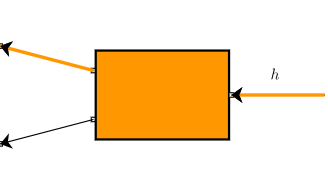
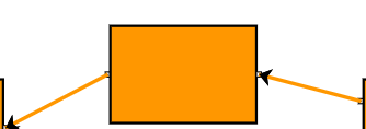
首先是最后一个黑盒橘盒即 输出的
每次反黑盒都是黑盒的输出变量通过黑盒的函数形式对输入变量逐个求偏导的过程。
进行第一个反黑盒backward计算,得到对两个输入变量各自的偏导数。 -
第二层
接下来假设先对上面那个节点进行处理,a自顾自地对z反黑盒(先拿到了偏导数用来乘,再让a对z求导,把用来乘的值和求导值乘起来)
再对下面黑盒处理,b对z反黑盒
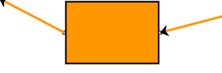
根据链式法则,为了将这一步两个反黑盒与前一步反黑盒结合起来、得到h对z的导数,除了前述“拿到偏导数用来乘”的步骤,还要把这一步两个反黑盒得到的值加起来。
(某一层有多个对相同变量的反黑盒,得到的导数要加起来)
- 第三层
最后一层反黑盒。拿汇合的导数值作为乘数,乘以z分别对x和y的偏导,就得到了结果:x.derivative和y.derivative,即h对x和y的偏导。
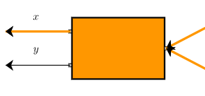
有趣的是,在以上的过程中,每个变量及中间变量(如h、a、b、x、y)都有保存的导数。
第一层反黑盒传入的导数是h对h,输出了h对a和h对b;
第二层反黑盒传入的导数是h对a和h对b,先计算了a对z和b对z,再输出了h对z;
第三层反黑盒传入的导数是h对z,先计算了z对x和z对y,再输出了h对x和h对y。
上述加粗的存储入以被求导变量为键的字典用于后续计算使用,而最后的变量(leaf variable, x和y)被存储(如x.derivative, y.derivative)。
Backpropagate Algorithm:反向传播算法
- Call topological sort to get an ordered queue
- Create a dictionary of Scalars and current derivatives
- For each node in backward order, pull a completed Scalar and derivative from the queue:
- a. if the Scalar is a leaf, add its final derivative (
accumulate_derivative) and loop to (1) - b. if the Scalar is not a leaf,
- a. call
.chain_ruleon the last function with - b. loop through all the Scalars+derivative produced by the chain rule
- c. accumulate derivatives for the Scalar in a dictionary
- a. call
之后实现了拓扑排序、实现了反向传播,再实现算子的backward,就搞定了这一段。
其中实现算子的backward时,需要什么变量,forward就存过来什么变量。(也可以为了节省计算而存入一些计算好的值,我这里直接传变量再算一遍了)
完结撒花。
Tensors
Tensor:把标量scalar换成张量Tensor,与Pytorch使用的数据结构保持一致
tensor_data
实现了tensor的索引部分,参考Pytorch的API确定相关功能。为了保证输出正确,相关命令结果均通过Pytorch运行后复制得到。
stride是在Tensor指定维度中从一个元素跳到下一个元素的步长,而shape是Tensor的形状。
也就是说stride是可以从shape推断得到的。
感觉stride是一个非常有用的思考方式,从多维到一维映射。一开始没看知识讲解,看了之后感觉醍醐灌顶。
- Strides is a tuple that provides the mapping from user indexing to the position in the 1-D
storage.contiguousmapping, is in the natural counting order (bigger strides left).
>>> a = torch.arange(6)
>>> b = a.view(2, 3)
>>> b
tensor([[0, 1, 2],
        [3, 4, 5]])
>>> b.stride()
(3, 1)
>>> b.shape
torch.Size([2, 3])
index方法:把元组形式的index转换为下标。
indices方法:产生n多个元组形式index的iterable,其中n是内部存储的数量。
    def indices(self) -> Iterable[UserIndex]:
        lshape: Shape = array(self.shape)
        out_index: Index = array(self.shape)
        for i in range(self.size):
            to_index(i, lshape, out_index)
            yield tuple(out_index)
把数字按照形状排列如果没有思路不妨找找规律。正如我们在CS61A中反复采用的方法,对应于某个初始值处理得到某一位,然后通过改变初始值再相同处理得到下一位,如是迭代。
# 0->(0,0) 5->(1,0) 10->(2,0) 14->(2,4), 当 shape=(3,5)
# 0->(0,0,0) 3->(0,0,3) 4->(0,1,0) 12->(1,0,0) 当shape=(2,3,4)
# out_index[-1] = ordinal % shape[-1]
# out_index[-2] = ordinal // shape[-1] % shape[-2]
# out_index[-3] = ordinal // shape[-1] // shape[-2] % shape[-3]
for i in range(len(shape) - 1, -1, -1): # 倒序
	out_index[i] = ordinal % shape[i]
	ordinal = ordinal // shape[i]
不妨读读从shape到stride转换的代码以加深理解:
def strides_from_shape(shape: UserShape) -> UserStrides:
    layout = [1]
    offset = 1
    for s in reversed(shape):
        layout.append(s * offset)
        offset = s * offset
    return tuple(reversed(layout[:-1]))
eg. (5, 2) -> (2, 1)
思考:
strides的最右侧维度,当前步长一定为1(offset的当前值为1),故layout初始化为[1]
strides的右数第二维,当前步长乘了shape最右侧维度,
右数第三维再乘了shape右数第二维维度,以此类推,
strides的最左维一定是乘了shape的左数第二维得到的。
permute方法用于重新排列维度:
import torch
x = torch.randn(2, 3, 5)
x_permuted = x.permute(2, 0, 1) # 使用permute函数重新排列维度
print(x_permuted.size()) # 输出: torch.Size([5, 2, 3])
这个很适合用列表推导式来写。因为列表推导式天然地可以根据某个顺序来重新排列列表。
例如将a按照order顺序排列,就是[a[i] for i in order]。
return TensorData(self._storage, tuple([self.shape[i] for i in order]), tuple([self.strides[i] for i in order]))
broadcasting
Rule 1: Any dimension of size 1 can be zipped with dimensions of size n > 1 by assuming the dimension is copied n times.
eg.
(3,) + (1,) = (3,)
(5, 1) + (5, 3) = (5, 3)
Rule 2: Extra dimensions of shape 1 can be added to a tensor to ensure the same number of dimensions with another tensor.
Rule 3: Any extra dimension of size 1 can only be implicitly added on the left side of the shape.
eg.
(3,) + (5, 3) = (1, 3) + (5, 3) = (5, 3)
(2, 3, 1) + (7, 2, 1, 5) = (1, 2, 3, 1) + (7, 2, 1, 5) = (7, 2, 3, 5)
Autograd
先看autograd的API效果:
>>> import torch
>>> tensor1 = torch.tensor([1.0, 2.0, 3.0], requires_grad=True)
>>> out = tensor1.sum()
>>> out.backward()
>>> print(tensor1.grad)
tensor([1., 1., 1.])
>>>
原因:执行了一个sum函数(当然梯度是不因tensor初始值发生变化的,只取决于执行的函数)
out = sum([x1, x2, x3]) = x1 + x2 + x3
所以out对x的梯度是[1., 1., 1.]
再比如说执行乘和求和两个函数,函数梯度再发生变化:
>>> tensor1 = torch.tensor([1.0, 2.0, 3.0], requires_grad=True)
>>> out = (tensor1 * 2).sum()
>>> out.backward()
>>> print(tensor1.grad)
tensor([2., 2., 2.])
It turns out that you can do most of machine learning without ever thinking in higher dimensions.
这里别的都好说,硬算就行,
permute函数的backward需要通过实验额外说明一下:
>>> x = torch.randn(2, 3, 4, requires_grad = True)
>>> y = x.permute(2, 0, 1)
>>> y.shape
torch.Size([4, 2, 3])
>>> loss = y.sum()
>>> loss.backward()
>>> x.grad.shape
torch.Size([2, 3, 4])
>>> x = torch.randn(2, 3, 4, requires_grad = True)
>>> loss = x.sum()
>>> loss.backward()
>>> x.grad.shape
torch.Size([2, 3, 4])
x先执行了permute,再执行了sum,之后执行backward。
从两个实验可以看出,无论是否执行permute,对完整过程执行backward得到的是一样的。这说明permute的backward事实上是一个逆向permute的过程,将gradient与输入张量对齐。
由此可以得到以下的实现:
    @staticmethod
    def backward(ctx: Context, grad_output: Tensor) -> Tuple[Tensor, float]:
		# 第一个是把grad_output按照a的shape和strides重排, 第二个是order的梯度为0.0
        (a,) = ctx.saved_values
        return Tensor.make(grad_output._tensor._storage, a.shape, a.strides, grad_output.backend), 0.0
之后2.4和2.5逐渐遇到一些神奇的bug,不知道是框架代码写错了还是我写错了。反正修改掉其中一者最后能跑就行。
Efficiency
Efficiency:使用numba并行和CUDA编程等方式提升效率。
Networks:已经开发出一个很简单的pytorch了,来拿它搞个卷积神经网络进行图像分类这种上游任务吧!
参考了:
- Minitorch项目文档
- numba的文档相关部分(Automatic parallelization with @jit)
- https://github.com/mukobi/Minitorch-Self-Study-Guide-SAIA
parallelization
Numba教程属于是。
比较:
def map(fn):
    # Change 1: Move function from Python to JIT version.
    fn = njit()(fn)

    def _map(out, input):
        for i in range(len(out)):
            out[i] = fn(input[i])

    # Change 2: Internal _map must be JIT version as well.
    return njit()(_map)
def map(fn):
	fn = njit()(fn)

	def _map(out, input):
		# Change 3: Run the loop in parallel (prange)
		for i in prange(len(out)):
			out[i] = fn(input[i])

	return njit(parallel=True)(_map)
三个优化目标:
- Main loop in parallel (用
numba.prange替代range) - All indices use numpy buffers (所有索引计算都使用ndarray,而非list或tuple)
- When
outandinare stride-aligned, avoid indexing(跳过索引计算,直接线性遍历)
ps. 搞不懂reduce的不要调用函数是啥意思。查阅了其他github fork的实现,都调用了函数。
这里有个搞笑的事情:在tensor_data/to_index函数的实现中,要加个trick:
把ordinal改成cur_pos,为了不是改变同一变量,加个0。
cur_pos = ordinal + 0 # 为了Module3并行, 不能修改循环变量的trick
for i in range(len(shape) - 1, -1, -1): # 倒序
	out_index[i] = cur_pos % shape[i]
	cur_pos = cur_pos // shape[i]
之后parallel_check三个函数都得到以下结果了:
------------------------------ After Optimisation ------------------------------
Parallel structure is already optimal.
--------------------------------------------------------------------------------
写这个task踩的一些坑:
- 把parallel=True关掉再看看。控制变量,从而确定是并行的问题、还是改函数的时候把函数逻辑改错了。
- 一点一点改。先跟原来的实现保持完全一致,然后慢慢加prange和快速路径等等,小步快跑,这样出错了可以发现问题在哪里。一口气全加上去了,报错还是得一点一点改。
- 到了并行,似乎很多时候调试器也不完全能解决问题。就像我拿pdb调到那里、自己调用相关函数跑发现addConstant确实把
[[0.00], [0.00]]加成[[5.00], [5.00]]了,明明跑的跟代码一模一样的函数,结果它并行起来就变成[0.00, 5.00]了。这是什么事嘛。
之后先把另外两个的parallel给关了,专心调map的问题。
Cannot determine Numba type
这里报了一个神奇的错误 Untyped global name 'exp': Cannot determine Numba type of <class 'function'>,需要回去改operators.py:
我在sigmoid实现中用到了同模块的exp函数,这是不被numba识别的,将其修改为math.exp或np.exp即可。
同理,在operators.py中的每个函数都不能互相依赖,而只能引用math或np库。
一开始:
def sigmoid(x: float) -> float:
    if x >= 0:
        return 1.0 / (1.0 + exp(-x))
    else:
        return exp(x) / (1.0 + exp(x))
修改后:
def sigmoid(x: float) -> float:
    if x >= 0:
        return 1.0 / (1.0 + math.exp(-x))
    else:
        return math.exp(x) / (1.0 + math.exp(x))
修改完保险起见把之前的测试用例再跑了一遍,没什么问题。
开着parallel=False先改完这个bug、task3.1可以全部通过。再把parallel=True打开跑跑看。
发现直接改prange解决不了问题。去读读numba的文档(Automatic parallelization with @jit)。
race
里面讲了一个race的案例。先拿串行测试一下正常情况:
>>> x = np.ones(4)
>>> n = x.shape[0]
>>> n
4
>>> y = np.zeros(4)
>>> for i in range(n):
...     y[:] += x[i]
...
>>> y
array([4., 4., 4., 4.])
如果写得不对,结果会如下:
>>> from numba import njit, prange
>>> @njit(parallel=True)
... def prange_wrong_result(x):
...     n = x.shape[0]
...     y = np.zeros(4)          # y = [0, 0, 0, 0]
...     for i in prange(n):      # 并行循环,i 同时跑
...         y[:] += x[i]         # 每个线程都在改 y 的全部元素
...     return y
...

>>> prange_wrong_result(x)
array([4., 4., 4., 4.])
>>> prange_wrong_result(x)
array([3., 3., 4., 4.])
>>> prange_wrong_result(x)
array([4., 4., 4., 4.])
>>> prange_wrong_result(x)
array([3., 2., 2., 2.])
>>> prange_wrong_result(x)
array([2., 2., 2., 2.])
我们可以查一下,发现numba会自动根据CPU核数把循环拆成多个线程来跑:
>>> from numba import config
>>> print("Numba 并行线程数:", config.NUMBA_NUM_THREADS)
Numba 并行线程数: 16
所以上述循环会拆成以下的效果,造成同时读写的冲突:
- 线程 A:执行 `y[:] += 1`
- 线程 B:执行 `y[:] += 1`
- 线程 C:执行 `y[:] += 1`
- 线程 D:执行 `y[:] += 1`
但如果通过 y += x[i] 等 Numba 能识别的 “规约操作”(reduction),Numba 会自动把 y += x[i] 转换成线程安全的加法,不会多个线程同时写同一个位置,不会race。
A reduction is inferred automatically if a variable is updated by a supported binary function/operator using its previous value in the loop body. The following functions/operators are supported:
+=,+,-=,-,*=,*,/=,/,max(),min(). The initial value of the reduction is inferred automatically for the supported operators (i.e., not themaxandminfunctions). Note that the//=operator is not supported because in the general case the result depends on the order in which the divisors are applied. However, if all divisors are integers then the programmer may be able to rewrite the//=reduction as a*=reduction followed by a single floor division after the parallel region where the divisor is the accumulated product. For themaxandminfunctions, the reduction variable should hold the identity value right before entering theprangeloop. Reductions in this manner are supported for scalars and for arrays of arbitrary dimensions. (numba文档)
因此排除发现,是我把out_index和in_index的初始化拿出循环的锅,出现race了。
修改后如下:
def tensor_map(
    fn: Callable[[float], float]
) -> Callable[[Storage, Shape, Strides, Storage, Shape, Strides], None]:
    def _map(
        out: Storage,
        out_shape: Shape,
        out_strides: Strides,
        in_storage: Storage,
        in_shape: Shape,
        in_strides: Strides,
    ) -> None:
        # 3. stride-aligned, 快速路径
        if (
            len(out_shape) == len(in_shape) and
            (out_shape == in_shape).all() and
            (out_strides == in_strides).all()
        ):
            for i in prange(len(out)): # 1. parallel
                out[i] = fn(in_storage[i])
        else:
            # 2. ndarray
            for out_i in prange(len(out)): # 1. parallel
                # 不要把out_index和in_index拿出循环, 不然会race
                out_index = np.empty(len(out_shape), dtype=np.int32)
                in_index = np.empty(len(in_shape), dtype=np.int32)
                to_index(out_i, out_shape, out_index)
                broadcast_index(out_index, out_shape, in_shape, in_index)
                out_pos = index_to_position(out_index, out_strides)
                in_pos = index_to_position(in_index, in_strides)
                out[out_pos] = fn(in_storage[in_pos])

    return njit(parallel=True)(_map)  # type: ignore
如法炮制、修改zip和reduce,成功通过task3.1。
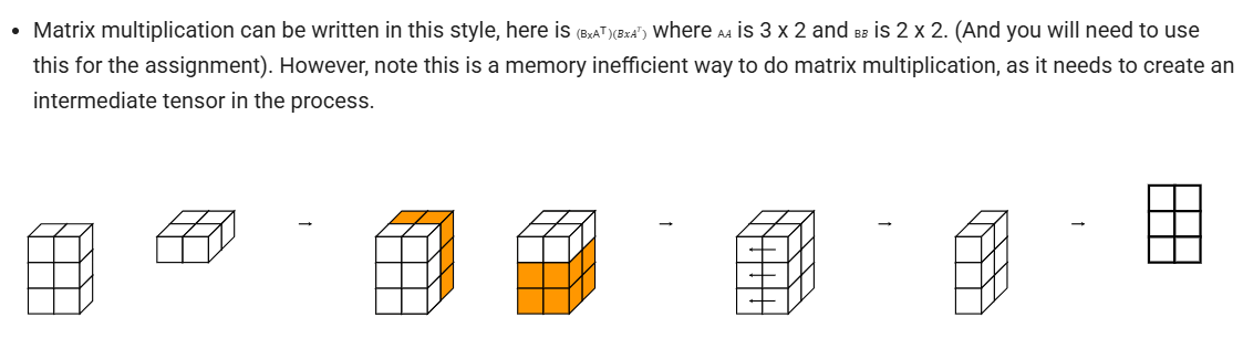
Matrix Multiplication
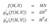
根据矩阵微积分的性质有:
优化要求:
- Outer loop in parallel
- No index buffers or function calls
- Inner loop should have no global writes, 1 multiply.
outer loop很好理解,就是遍历结果矩阵index的那个loop,这个肯定是prange就搞定了的。
第二行还是没听懂,为了思考方便还是直接调用之前实现的to_index之类的函数了。
第三个是理所应当的,按照numba优化的写法把reduction变量写在外面、里面+=。
关于numba.cuda
之后看了一眼 projects/run_fast_tensor.py ,发现我用pip安装的numba==0.60.0没有numba.cuda,于是pip uninstall了一下,又用conda安装了numba和cudatoolkit。
pip uninstall numba
conda install numba==0.60.0 cudatoolkit -c conda-forge -y
然后拿以下指令查了一下:
>>> from numba import cuda
>>> print(cuda.gpus)
<Managed Device 0>
感觉是minitorch的代码和我numba版本不匹配,把numba.cuda.is_available()改了一下:
from numba import cuda
if cuda.gpus:
    GPUBackend = minitorch.TensorBackend(minitorch.CudaOps)
CUDA operations and Matrix Multiplication
未进行学习,直接在代码中参考了github上可通过测试的开源实现。
Task3.3: atgctg/minitorch: Solutions for http://minitorch.github.io
Task3.4: feimos32/Minitorch-Learning-Introduction: (已完结)斯坦福大学机器学习项目MiniTorch解读——《MiniTorch 学习全攻略》 的随书源码。
(推荐:MiniTorch-学习全攻略.pdf)
附: 基于Pytorch代码,讲讲反向传播和计算图
以下代码选取自PyTorch官方的 Quickstart — PyTorch Tutorials
省略了import,数据集加载,设置DataLoader,建立模型,设置损失函数和优化器。
def train(dataloader, model, loss_fn, optimizer):
    size = len(dataloader.dataset)
    model.train() # 将模型设置为训练模式
    for batch, (X, y) in enumerate(dataloader):
        X, y = X.to(device), y.to(device)

        # Compute prediction error
        pred = model(X) # 模型前向传播, 得到预测值
        loss = loss_fn(pred, y) # 根据预测值和实际值, 得到loss

        # Backpropagation
        loss.backward() # !Autograd主要干了这个函数的事情!
        optimizer.step() # 优化一轮参数
        optimizer.zero_grad() # 将梯度清零

        if batch % 100 == 0:
            loss, current = loss.item(), (batch + 1) * len(X)
            print(f"loss: {loss:>7f}  [{current:>5d}/{size:>5d}]")
def test(dataloader, model, loss_fn):
    size = len(dataloader.dataset)
    num_batches = len(dataloader)
    model.eval()
    test_loss, correct = 0, 0
    with torch.no_grad(): # 为了加快推理, 所有前向操作都不计算梯度
        for X, y in dataloader:
            X, y = X.to(device), y.to(device)
            pred = model(X) # 上面设置后, 这里面的每一步前向操作都不计算梯度
            test_loss += loss_fn(pred, y).item()
            correct += (pred.argmax(1) == y).type(torch.float).sum().item()
    test_loss /= num_batches
    correct /= size
    print(f"Test Error: \n Accuracy: {(100*correct):>0.1f}%, Avg loss: {test_loss:>8f} \n")
我们知道,在前向传播的同时也建立了计算图。用以下数值例子举例。
ps. 数值例子由GPT生成,可能存在计算错误。
单变量标量函数
前向传播:
计算图:
    x=1     2
     \     /
      + --> a=3
        \
         \
          **2 --> y=9 --> L=9
由,依次用计算的偏导数。
首先计算 ,
再计算
最后计算
可见每一步的共同点:以计算 为例,
都是把上一步的梯度计算结果(如 )拿过来,乘以这一步计算出的梯度(如 )。
我们可以把正向的过程看作正向的一个黑箱操作(即构造的计算图),
由上一步传播过来的值进行了函数运算得到另一个值、传播的是函数值,
而反向的过程看作反向的一个黑箱操作(即计算图的逆向),
由上一步传播过来的导数值乘以当前步的求导运算得到另一个导数值,传播的是导数值。
多变量标量函数
前向传播:
计算图:
  w=2   x=3       b=1
   \   /          |
    * --> a=6     |
      \          /
       + --> z=7
         \
          \
           **2 --> L=49
这里重点关注两个点:一是两个变量的加法,二是两个变量的乘法。
将两个变量加在一起时(如),对每个变量的偏导值均为1。所以要得到对每个变量的偏导,只需把上一步传播过来的值乘以1即可。
将两个变量乘在一起时(如),对求导得到的是的值,反之对求导得到的是的值。所以要得到对每个变量的偏导,只需把上一步传播过来的值乘以另一个变量即可。这一事实也会运用到后面的矩阵乘法上。
矩阵乘法
前向传播:
计算图:
     X        W
      \      /
       @ --> h (2x2)
         \
          \
           sum(h²) --> L=166
反向传播:要求 和 。
根据矩阵微分的知识,
ps. 这里的矩阵乘法反向传播同样遵循“L对某个变量求导,就是拿传播值乘以另一个变量”,与前述“多变量标量函数”部分有共通之处。
MiniTorch相关代码参考
以 ScalarFunction 中的 Log 函数举例:
在forward时,传入 ,计算 并返回。
在backward时,传入 即上一步得到的导数,计算它与本步骤的导数 ( ) 的乘积并返回,即得到误差函数 对变量 的导数。
为了在backward时计算本步骤的导数( ),需要在forward中将 的值记入Context中,从而在backward计算时取出。
class Log(ScalarFunction):
    "Log function $f(x) = log(x)$"

    @staticmethod
    def forward(ctx: Context, a: float) -> float:
        '''保存a, 计算log(a)并返回'''
        ctx.save_for_backward(a)
        return operators.log(a)

    @staticmethod
    def backward(ctx: Context, d_output: float) -> float:
        '''取出保存的a, 根据传回的d_output, 计算d_output / f\'(x)并返回, 即d_output / a'''
        (a,) = ctx.saved_values
        return operators.log_back(a, d_output)
总结
由上述案例可知,计算图是描述前向传播、反向传播过程的一个通用手段。
它将反向传播中每一步的导数计算简化为上一步传播的值 乘以 这一步的导数,
通过记录前向传播中经历的函数过程及相应变量的值,达成了反向传播的计算。
前向传播即是由输入变量经过模型(即一系列的函数操作)得到输出变量的过程。
(输出变量经历激活函数,与实际变量通过损失函数计算出损失)
反向传播即是由损失值逆着模型(即一系列的求导运算)计算出损失函数对各个输入变量的偏导数。
(得到偏导数是为了优化器可以采用梯度下降等方式更新模型参数)
在这样观察了之后,对PyTorch的训练与推理的函数过程就了解得比较完整了。
edit time: 2025-07-02 17:07:11 (Fundamentals√)
edit time: 2025-07-02 17:54:05 (ML Primer√)
edit time: 2025-07-07 23:33:57 (AutoDiff√)
edit time: 2025-07-15 17:18:18 (Tensors√)
edit time: 2025-07-23 22:29:56 (Efficiency√)
edit time: 2025-08-03 22:09:45 (附: 基于Pytorch代码,讲讲反向传播和计算图√)